Energy analysis in ice hockey arenas and analytical formula for the temperature prole in the ice pad with transient boundary
conditions
Andrea Ferrantellia, Klaus Viljanenb and Jarek Kurnitskia,b
aTallinn University of Technology, Department of Civil Engineering and Architecture, 19086
Tallinn, Estonia;bAalto University, Department of Civil Engineering, P.O.Box 12100, 00076
Aalto, Finland
ARTICLE HISTORY Compiled May 3, 2019 ABSTRACT
The energy eciency of ice hockey arenas is a central concern for the adminis-trations, as these buildings are well known to consume a large amount of energy. Since they are composite, complex systems, solutions to such a problem can be approached from many dierent areas, from managerial to technological to more strictly physical.
In this paper we consider heat transfer processes in an ice hockey hall, during operating conditions, with a bottom-up approach based upon on-site measurements. Detailed heat ux, relative humidity and temperature data for the ice pad and the indoor air are used for a heat balance calculation in the steady-state regime, which quanties the impact of each single heat source. We then solve the heat conduction equation for the ice pad in transient regime, and obtain a generic analytical formula for the temperature prole that can be used in practical applications.
We then apply this formula to the resurfacing process for validation, and nd good agreement with an analogous numerical solution. Since it is given with implicit initial condition and boundary conditions, it can be used not only in ice hockey halls, but in a large variety of engineering applications.
KEYWORDS
transient heat conduction; cooling; theoretical models; analytical solutions; ice rinks; energy eciency
1. Introduction
A well-known major preoccupation of contemporary building research is the energy e-ciency of buildings, which is subject to increasingly stringent requirements set by man-ufacturers and international institutions (European Parliament (2010); Butera (2013)) under ecological and economical motivations.
In this context, ice hockey arenas are fairly demanding systems, infamous for con-suming a very large amount of energy that approaches ∼ 1800 MWh per year. In particular, according to several studies (see e.g. Karampour (2011); Räikkönen (2012); Ferrantelli et al. (2013)) refrigeration is responsible for nearly 43 percent of the total
energy consumption of the ice hockey hall. Process optimization and energy eciency have therefore increased their role of key research concepts on very diverse, yet cor-related aspects of energy management. These can range from the concrete pad design as in Haghighi et al. (2014), to the air distribution and ventilation (Yang et al. (2000, 2001)) and their eect on the overall heat balance, as addressed by Palmowska and Lip-ska (2018); Toomla et al. (2018); Taebnia et al. (2019), as well as the exergoeconomic analysis performed by Erol et al. (2017).
Furthermore, these types of buildings constitute a challenging setup for studies in building physics, due to the diverse physical processes often concurring to each other, which take place in the environment. For instance, ventilation and air conditioning in such large and complex systems are an intriguing eld of study, as illustrated by Caliskan and Hepbasli (2010); Daoud et al. (2008); Teyssedou et al. (2013). More-over, opportunities for energy conversion (Zhao et al. (2016)), electrical energy storage (Chen et al. (2013)) and passive measures such as air transport and water vapour control (Amirifard et al. (2018)) nd in this context an interesting eld of study and application. All in all, very dierent types of solutions can be realized for promoting the energy saving by increasing the overall system eciency, see e.g. Castellani et al. (2017) for solar energy storage and Castellani et al. (2019) for pure methane collection. The various contributions to the energy balance in such a complex system are usually addressed numerically. Heat and mass transfer processes occur both above and inside the large ice/concrete slab forming the ice rink, and have been thoroughly studied for at least a couple of decades now, see for instance Negiz et al. (1993); Hastaoglu et al. (1995) and more recently Teyssedou et al. (2009). Computational Fluid Dynamics (CFD), see e.g. Ohba and Lun (2010) for a review, is a useful tool in this sense. CFD simulations in 2D were performed under steady state conditions in Bellache et al. (2005), where velocity, temperature and absolute humidity distributions were predicted for an indoor ice rink with heating provided by ventilation. The numerical model was then extended to transient processes by the same authors in Bellache et al. (2006), adding calculations of heat transfer through the ground, energy gains from lights and resurfacing eects. A CFD numerical analysis of the radiative component induced by thermostatically controlled radiant heaters has been considered in Omri et al. (2016), tracking the heat ow and temperature inside the ice hall, together with the heat uxes into the ice pad. Regarding analytical solutions, the literature is far less abundant mostly because of evident technical diculties. General solutions for coupled heat transfer do exist however, since they pertain more general cases such as building foundations and ra-diant oors. Somrani et al. (2008) used the Interzone Temperature Prole Estimation (ITPE) method developed in Krarti (1999), considering an ice pad with constant upper boundary condition (the air temperature just above the ice surface), laying over sand, insulation, a soil layer with time-varying temperature and a water table with constant temperature.
More recent investigations concentrate on large scales, and consider the entire ice hall in view of numerical integration towards energy optimization, see for instance Mun and Krarti (2011). As an example, Tutumlu et al. (2018) formulated a model for assessing the thermal performance of a cooling system consisting of an ice rink, a chiller unit and a spherical thermal energy storage tank. Computing the ice rink heat gain and the energy consumption of the chiller unit, they were able to determine the operation time of this large system in function of indoor conditions, storage tank and chiller characteristics.
literature. Additionally, in this specic context there currently exists a lack of heat transfer formulas which are easy to apply to practical design problems.
In this paper we try to address these issues by considering the topic on a smaller scale, i.e. an ice pad element, by means of a bottom-up approach based on measurements. For the rst time in the literature, we report detailed measurements of the heat ux as well as ice temperature at the surface and at the bottom of the ice pad during resurfacing. These constitute the time-dependent boundary conditions (b.c.) for an analytical temperature prole along the ice slab depth which we accordingly compute. Though the derivation is rather involved, we recast the resulting temperature prole in function of the boundary conditions as a simple formula which can be easily im-plemented in common computational software. This is another novelty of this paper, aimed at immediate practical usage. Our main purpose is indeed to provide a concise reference for practical applications in ice hockey halls, by means of an easily applicable formula for the ice pad temperature together with comprehensive data of heat ux, air stratication and humidity at various heights in the ice hockey arena.
We choose the resurfacing stages because they are the most complex and energy consuming phases of the operational cycle of an ice hockey hall, due to the large amount of heat transferred to the ice pad in a relatively short time. This aects importantly the eciency and energy consumption of the refrigerating system, and here we aim at nding applicable quantitative knowledge to aid e.g. system control and space heating investigations.
Though obtained for a specic case-study, our measurements can be applied to the majority of standard ice hockey halls, for instance in the development of new control methods for ice rink cooling systems (see for instance Lü et al. (2014, 2015)). Our ndings also help in developing methods to reduce the indoor temperature stratication as suggested by Taebnia et al. (2019), or to collect a portion of the heat generated and reuse it in the ice hockey hall. Moreover, the temperature prole formula we obtain is very general and is not limited to ice hockey arenas; rather, it can be applied to other heat conduction processes with transient boundary conditions.
The present paper is organized as follows: Section 2 reports the experimental setup and measurements, as well as an energy balance analysis which is validated with exper-imental data. We examine the heat ux on the ice pad, the indoor air relative humidity (RH) in its proximity and the temperatures at surface and at the ice/concrete interface during a typical day of operation.
In Section 3 we use the eld measurements to estimate the diverse contributions to the heat load over the ice pad in the steady state conditions immediately preceding the resurfacing, considering convection, condensation and radiation. An analytical for-mula for the ice pad temperature in transient conditions is then derived in Section 4. Our results are summarized and further discussed in the Conclusions, and nally in Appendix A we apply our formula to the calculation of the temperature prole inside the ice pad during resurfacing, validating it with the initial data.
2. Ice hockey hall and temperature measurements
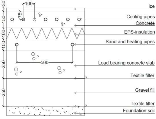
Figure 1. A portion of the ice rink oor structure considered.
is usually done by means of resurfacing machines. These devices rst shave the ice, then brush it and eventually spread a thin layer of new water on the surface.
At each maintenance cycle, 300 to 800 liters of water are used, corresponding to a 0.25-0.5mm thick water layer. The water cooling and freezing processes generate a sudden increase in the ice temperature, which lowers the cooling eciency of the refrigerating system, thus increasing the operational costs of the ice hall. Accurate analysis of this phenomenon is then important to optimize the refrigeration process and to achieve overall energy saving.
The eld study discussed in this paper was carried out at the Reebok Arena in Leppävaara, Finland, during summer conditions1. The ice hall has two identical ice rinks of size 1624 m2 each. There are no major stands in the hall and the ventilation air ow rate varies between 3-6 m3/s during the year. The refrigeration system is indirect, with ammonium as the refrigerant and ethylene glycol as the brine.
Consider now a modular component of the ice/concrete slab as in Fig.1: ice 30mm, concrete slab 150mm with brine pipes at the middle, EPS-insulation 100mm, sand 100mm with frost pipes and a load bearing concrete slab 250mm. The coecient of performance for the refrigeration system is ∼ 1.6 on the average, as documented in Ferrantelli et al. (2013).
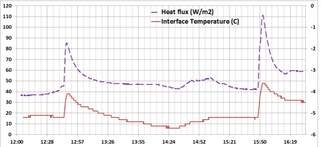
We focus on the rst resurfacing process in Fig.2, corresponding to the peak near 12:45. The ice surface has an initial surface temperature TS ∼-4.5°C, the whole ice
pad is at−5°C on the average. During resurfacing,mw=450kg of water at temperature
Tw=40°C are spread on the ice surface at t=0s. The entire process consists of three
phases:
1. cooling of the water layer by contact with the ice pad, convection and radiation with the surroundings,
2. complete freezing of the water by the same processes,
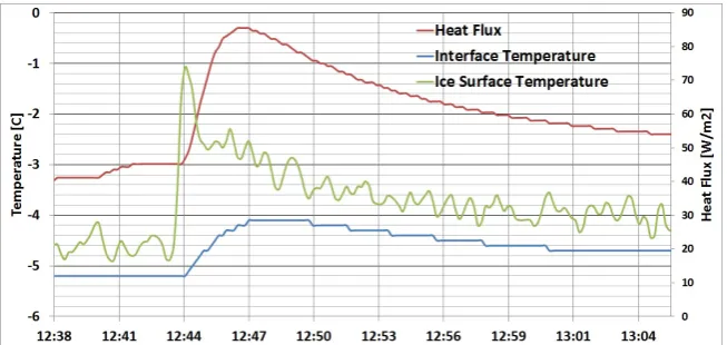
3. cooling of the new ice from Tf reeze=0°C to Tice ∼-4°C (see Fig.3). A thermal
Figure 2. Measurements of temperature and heat ux at the ice/concrete interface.
Moreover, heat ux and temperature are measured with a heat ux plate and a pt-100 temperature sensor installed at the ice/concrete interface in the slab, as shown in Fig.2. The according data are plotted in Fig.3.
The physical properties of water are evaluated at the lm temperature Tf=20°C,
implying a specic heat cp,w=4.182 kJ/kgK. Since mw=450kg of water are spread on
the ice, the average thickness is only
x= mw
ρA = 0.28mm , (1)
which is anyway just an indicative value, as the precision of the resurfacing machine is not high enough. The size of the ice rink isA=1624 m2, hf s=338 kJ/kg is the water
latent heat of freezing andcp,i=2.05 kJ/kgK is the specic heat of ice atT ∼0°C. The
water chilling and freezing loads are thus obtained as follows,
Qw= [mw[hf s+cp,w(Tw−0) +cp,i(0−Tice)]] (2)
= 231.21M J; qw = 142.37
kJ
m2 , (3)
Q1=mwcp,w(Tw−0) = 75.28M J; q1 =
Q1
A = 46.4 kJ
m2 , (4)
Q2=hf smw = 152.1M J; q2=
Q2
A = 93.7 kJ
m2, (5)
Q3=mwcp,i(0−Tice) = 3.69M J; q3 =
Q3
A = 2.27 kJ
m2 , (6)
where Tice is the temperature of the frozen resurfacing water under the new steady
state conditions. The theoretical heat load Eq.(3) is consistent with the literature, as in Seghouani et al. (2009, 2011).
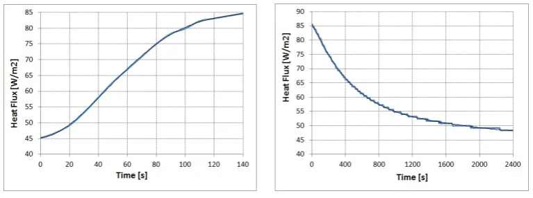
Let us verify immediately that the theoretical heat ux in (3) is consistent with the measurements at the ice/concrete interface in Fig.3. The integral of the heat ux curve is the total heat transferred during the resurfacing, to be compared with Eq.(3). For better precision, we split the curve into three contributions: two polynomials2 plotted in Fig.4 (R2 = 0.9997) and Fig.5 (R2 = 0.9991), and a constant value q˙max=85.4839
2At rst sight the plot in Fig.5 seems to suggest an exponential, however the accuracy is that case would be
Figure 3. Heat ux and temperatures during the water chilling and freezing.
W/m2, corresponding to the narrow (∆t ∼ 30s) plateau at the top of the curve in
Fig.3.
If q˙A is the heat ux rate for the rst contribution and q˙B the ux for the second
curve, we obtain the following expressions:
˙
qA(t) = 3×10⁻⁷t4−10−4t3+ 0.0106t2+ 0.0414t+ 45.191, (7)
˙
qB(t) = 3×10⁻¹²t4−2×10⁻⁸t3+ 5×10⁻⁵t2−0.0647t+ 85.873. (8)
Integrating the above over the respective time intervals gives
qA= Z 140
0
˙
qA(t)dt= 10.05
kJ
m2, (9)
qB = Z 2300
0
˙
qB(t)dt= 127.88
kJ
m2, (10)
to which we add the heat transferred at the peak, namely
qmax= 85.4839
W
m2 ×∆t[s] = 2.57
kJ
m2 . (11)
Consistently with point 3. of the resurfacing process, the upper limit of the integral (10) coincides with the instant when the ice surface temperature reachesTice=-4°C.
The total heat transferred to the ice pad during the three phases of resurfacing in Eq.(3) is therefore estimated as
qexp = 140.49
kJ
m2 . (12)
This is very close to the theoretical mean value in Eq.(3), holding as
qw = 142.37
kJ
Figure 4. Interpolation curve for Eq.(9). Figure 5. Interpolation curve for Eq.(10).
we nd indeed
∆q≡qw−qexp = 1.88
kJ
m2, %(∆q) = 1.32%, (14)
which is fairly satisfactory and veries the consistency of the theoretical and measured heat load3.
2.1. Indoor air measurements
Regarding the air temperature and RH, we used dierent sets of data obtained in dierent sessions. One set of data was obtained at 0.04m, 0.1m and 0.24m above the ice rink with accuracy ±2% for 0-90% relative humidity and ±3% for 90-100% RH. The accuracy of the temperature measurement was±0.4°C. Later on, additional
measurements were made at 0.6m, 1.2m, 1.8m and 2.2m above the ice with PT-100 temperature sensors, with accuracy±0.5°C. Moreover, the temperature was measured
at 5.0m and 8.3m height with an accuracy of ±0.5°C. All measurements were done
with ∆t=10s interval and lasted approximately four hours. The probes set at 0.04-2.2m height were set up in a metal holder standing above the ice; this was located at one corner of the ice rink, 1m from the edge of the ice pad.
Further measurements were later performed at 0.005m, 0.01m, 0.04m, 0.1m, 0.24m and 5m height over the ice with dierent probes, to substantially reduce the errors. These now held as±0.3% for RH and±0.1°C for the temperature, with an according ±0.02 g/m3 error for the computed absolute humidity. While during resurfacing and
skaters' practice such high accuracy is not necessarily needed, as the stratication is erased by the air mixing, under steady state conditions this is crucial for the energy balance estimate we perform in Section 3. These later results are listed in Table 1.
All data were collected at one instance after the sensors had became steady. The probes at 0.005-0.24m height were again set up in a metal holder over the ice. Two locations of the holder were used, at the corner of the ice rink and closer to the centre of the ice pad, at approximately 8m from the edge where also the heat ux plates were installed and thermal camera measurements were taken.
The air temperature at 0.6m-8.3m over the ice is plotted in Fig.6, while that at 0.04m-0.24m in Fig.7. All the other data are shown in Table 1.
3This is precise enough for our purposes, notice anyway that one has some freedom in setting the upper limit
The plots show that, as expected, the air temperature above the ice rink is strongly stratied, see Fig.6, Fig.7 and Table 1, consistently with Toomla et al. (2018). The temperature at 0.6m height is 2°C and 10°C at 5m. Interestingly, by virtue of the mixing eect of the ventilation system supplying warm air at 25°C at 5m above the ice, the highest temperature is at 5m instead of 8.3m (Fig.6). Furthermore, the stratied air temperature at 0.6-2.2m turns into a more uniform temperature when the skaters enter the ice rink at 14:30 and start mixing the air layers.
The measured relative humidity (RH) and absolute humidity (AH), listed in Table 1, suggest that above the ice rinks the RH is uniform at heights 0.005m - 0.24m over the ice and distinctly lower farther from the ice pad. The relative humidity is higher above the ice than in the other parts of the space, yet it never reaches 95-100%.
The measurements did not imply any signicant dierences in temperature or rel-ative humidity depending on the location over the ice pad, either corner or centre, in agreement with Taebnia et al. (2019).
Figure 6. Air temperature above the ice during resurfacing and skaters activity.
Table 1. Air temperature, relative humidity (RH) and absolute humidity (AH) as measured at dierent heights from the ice pad surface during steady state conditions.
Height over the ice [±0.005 m] T [±0.1 °C] RH [±0.3%] AH [±0.02 g/m3]
5.0 4.2 77.2 4.98
0.24 -0.8 90.2 4.15
0.1 -2.2 89.6 3.76
0.04 -2.7 89.3 3.59
0.01 -3.1 88.1 3.45
0.005 -3.5 88.2 3.36
3. Energy balance and ice temperatures before resurfacing
In this section we use the eld measurements to compute some estimates of the heat loads on the ice pad before resurfacing. We consider convection, condensation and radiation. In this case the heat transfer is steady state in good approximation, so this is easy to accomplish. Even though it is dicult to obtain very precise values, this shows well the various factors concurring to the overall energy balance on the ice hockey rink. Consider rst Fig.2 and Fig.3 before resurfacing, namely before∼12:43. The heat
ux through the ice pad and the ice temperature, both measured at the ice/concrete interface, are respectivelyq˙=41.85 W/m2 (average) andTI=-5.2°C. The ice pad
thick-ness is on the average L=30mm. We can derive the ice temperature at surface very easily, ifkice=2.25 W/mK,
TS =TI+
L kice
˙
q =−4.64◦C, (15)
which is consistent with the ice surface temperature given in Fig.3.
The heat ux on the ice track surface is the sum of several contributions,
˙
q= ˙qrad+ ˙qconv+ ˙qwvcond+ ˙qlamp
=hrad(Tceiling−TS) + (hconv+hwvcond)(Tin−TS) + ˙qlamp, (16)
namely thermal radiation from the ceiling, convection and water vapor condensation at the surface, and heat load from the lighting system. For simplicity, we neglect the thermal radiation from the vertical walls and from the audience stands. These should not give a relevant contribution, since each ice rink is much larger than the walls' height, and ice pad and walls are separated by several meters of empty oor. Additionally, the ice surface temperature was measured at ∼8m from the edge towards the ice pad's
centre (Section 2.1), thus farther away from the walls (see also Karampour (2011)). This is fairly dierent from the situation addressed by Omri et al. (2016), in a much smaller ice hockey hall.
For convection we useTin=T(0.005m)= -3.5°C, see Table 1. Thus the heat transfer
coecient takes into account both natural convection and a correction given by forced convection, following ASHRAE (2010)
hconv= 3.41 + 3.55V = 3.94
W
corresponding to V = 0.15m/s for the air ow right on top of the ice Räikkönen (2012). The convection heat ow is therefore
˙
qconv =hconv(Tin−TS) = 4.49
W
m2. (18)
The radiation heat transfer coecient is written instead as
hrad =ε12σ(Tceiling2 +Tice.sur2 )(Tceiling+TS) = 1.39
W
m2K, (19)
whereTceiling=18°C and the resulting emissivity is computed according to ASHRAE
(1994),
ε12=
1 Fci
+
1 εceiling
−1
+Ac Ai
1 εice.sur
−1
−1
. (20)
The view factor between ceiling and ice isFci= 0.68, while emissivitiesεice.sur = 0.98
and εceiling = 0.33 for ice surface and ceiling (a load bearing sheet of galvanized steel
whose portion above the ice rink has areaAc=2600 m2) are respectively used, following
Räikkönen (2012). These giveε12= 0.278.
One must also take into account the radiative heat transferred to the ice pad by the lighting system. The lamps in Leppävaara are metal halide, which implies a contribu-tion of 400W per lamp. The porcontribu-tion of this power that is turned into heat is nearly 62%, as given by the manufacturer Osram GmbH (2014). Using the upper limit for the heat generation for 40 lamps gives the following contribution:
˙
Qlamp= 9.92kW , (21)
corresponding to the following heat ux,
˙ qlamp =
˙ Qlamp
A = 6.11 W
m2 . (22)
The water vapor condensation heat load is computed following Granryd (2005),
˙
qwvcond=hd(Tin−TS)
W m2
, (23)
where the heat transfer coecient for condensation hd is calculated from
hd = 1750hconv
∆p
∆T , [p] = [atm]
∆p = ϕinpin−ps. (24)
Figure 8. Contributions to the heat load over the ice pad in steady state conditions, Eq(27).
surface, as in Table 1. The saturation pressures are calculated from (here [T]=[°C])
pin = 105exp
17.391− 6142.83
273.15 +Tin
, (25)
ps = 105exp
17.391− 6142.83
273.15 +TS
. (26)
We thus obtainhd= 0.9W/m2Kandq˙wvcond= 1.03W/m2. By substituting this result
into (16), together with Eqs.(18), (19) and (20), and adding also (22), we get
˙
q = ˙qrad+ ˙qconv+ ˙qwvcond+ ˙qlamp= 31.25 + 4.49 + 1.03 + 6.11 = 42.87
W
m2 , (27)
that overestimates only slightly the measured value 41.85W/m2. The percentage of each contribution is listed in Fig.8. Now we focus on the ice/concrete pad and consider only conduction. The steady-state conditions provide for the heat ow inside the slab
˙
q = TS−Tp Rtot
= TS−Tp Rice+Rconc
, (28)
whereTp is the temperature at the top of the pipes and the thermal resistances of the
ice and concrete slabs are written as
Rice=
L kice
= 1.33×10⁻²Km
2
W , (29)
Rconc=
d kconc
= 1.67×10⁻² Km
2
W , (30)
pipesTp is then estimated from
˙
q= 41.85W/m2 = TS−Tp Rtot
, (31)
which givesTp=-5.9°C and can be cross-checked with heat balance inside the concrete
slab only,
˙
q = TI−Tp Rconc
. (32)
This in fact returnsq˙= 41.92W/m2 ≈41.85W/m2.
Let us nally check the agreement between the thermal camera measurement and the result (15) for the ice surface temperature. The heat transfer via conduction inside the ice pad is written as
˙ qI =
TS−TI
Rice
. (33)
Since this also must be equal to q˙, namely q˙I = ˙q = 41.85 W/m2 because of the
steady state conditions, substituting and solving with respect to the temperature at the ice/concrete interface we get
TI =TS−Riceq˙=−5.2◦C, (34)
that is indeed consistent with the measured value.
4. Analytical temperature prole for the ice pad
In this section we derive an analytical formula for the temperature prole of the ice pad Tice(t, x), which can be used under any specic situation occurring in the ice hockey
hall. The problem consists of solving the heat equation
∂u ∂t =αI
∂2u
∂x2, (35)
where 0 < x < L = 30mm, and αI is the thermal diusivity of ice, with the
time-dependent boundary conditions
u(0, t) =TS(t), (36)
u(L, t) =TI(t), (37)
and the initial condition
u(x, t= 0) =f(x) = 18.67(0.03−x)−5.2, (38)
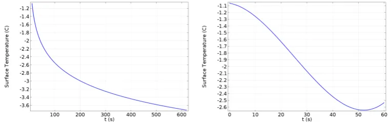
Figure 9. Interpolation of the surface tempera-tureTS(t)overt≤620s.
Figure 10. Interpolation of the surface temper-atureTS(t)fort <60s.
The boundary conditions are in general given by the measurements. In this specic case,TS(t) is computed at the ice surface (at the water/ice interface) andTI(t)at the
ice/concrete interface. They both are illustrated in Fig.3.
To obtain the analytical form of TS(t), we interpolate the temperature of the ice
pad at the surface. The overall trend, including the entire curve from the beginning of resurfacing tot= 620s, is clearly logarithmic. It gives the equation
TS(t) =−0.641 ln(t) + 0.4016 t[s]≤620. (39)
If instead we consider e.g. only the rst minute, the surface temperature becomes
TS(t) = 2×10⁻⁵t3−0.0015t2−0.0065t−1.0633, t[s]≤60. (40)
These interpolations are given in Figs.9 and 10. The temperature raise in the last 10s is due to the third order polynomial (this is non physical, still it remains within the experimental error and does not aect the result sensibly). The formula for the ice-concrete interface temperature, in the rst approximation, is also a simple third-order polynomial obtained from the eld measurements (Fig.3),
TI(t) = 6×10⁻⁶t3−3×10⁻⁴t2+ 4.3×10⁻³t−5.2071, (41)
which is plotted in Fig.12. We will apply these in the Appendix.
To solve the Cauchy problem given by Eqs.(35), (36), (37) and (38), we adopt the method of Eigenfunctions Expansions detailed in Titchmarsh (1962a,b); Hahn and Ozisik (2012) as follows. First impose the following Ansatz
w(x, t) =TS(t) +x
TI(t)−TS(t)
L
, (42)
that implies
w(0, t) =TS(t), (43)
w(L, t) =TI(t). (44)
Figure 11. Initial conditionf(x). Figure 12. Interpolation of the interface
tem-peratureTI(t)fort <60s.
u(x, t) =w(x, t) +v(x, t), (45)
and substitute this expression in the Cauchy problem. We obtain
vt=αIvxx−wt, (46)
where we have simplied the derivatives notation, with the Dirichlet boundary condi-tions v(0, t) = v(L, t) = 0and the initial condition v(x,0) = f(x)−w(x,0). Now use the Eigenfunction expansion
v(x, t) = ∞ X
n=1
ˆ
vn(t) sin (λnx), (47)
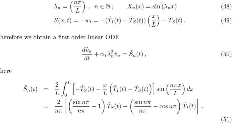
to separate space and time dependence. The eigenvalues and eigenfunctions associated to the Dirichlet b.c. are
λn=
nπ
L
, n∈N; Xn(x) = sin (λnx) (48)
S(x, t) =−wt=−( ˙TI(t)−T˙S(t))
x
L
−T˙S(t). (49)
Therefore we obtain a rst order linear ODE
dˆvn
dt +αIλ
2
nvˆn= ˆSn(t), (50)
where
ˆ
Sn(t) =
2 L
Z L
0 h
−T˙S(t)−
x L
˙
TI(t)−T˙S(t) i
sinnπx L
dx
= 2
nπ
sinnπ nπ −1
˙ TS(t)−
sinnπ
nπ −cosnπ
˙ TI(t)
,
(51)
following solution,
v(x, t) = ∞ X
n=1
Z t
0
dτ e−αIλ2n(t−τ)Sˆ
n(τ) +e−αIλ
2 ntc
n
sin (λnx), (52)
where the coecients
cn=
2 L
Z L
0 n
f(x)−h(TI(0)−TS(0))
x
L
+TS(0) io
sin
nπx
L
dx , (53)
are given by the initial conditionu(0, x) =f(x).
Putting everything together, we can now write the analytical temperature prole for the ice pad Eq.(45) as
u(x, t) = Tice(x, t) = [TI(t)−TS(t)]
x
L
+TS(t)
+ ∞ X n=1 Z t 0
dτ e−αIλ2n(t−τ)Sˆ
n(τ) +e−αIλ
2 ntc
n
sin (λnx), (54)
that constitutes a novel result of this paper. This is a completely general formula, with implicit initial conditionf(x) and b.c.TI(t) and TS(t).
The above clearly reduces to the ice temperature TS(t) at the surface for x = 0,
while it is slightly less immediate to verify that (54) is consistent with the temperature at the bottom of the ice pad TI(t)for x=L. In this case we get
u(L, t) = Tice(L, t)≡TI(t) = [TI(t)−TS(t)] +TS(t)
+ ∞ X n=1 Z t 0
dτ e−αIλ2n(t−τ)Sˆ
n(τ) +e−αIλ
2 ntc
n
sin (λnL). (55)
Recall now that
λn=
nπ
L , (56)
which implies
−2TS(t)
∞ X
1
sin (λnL)
nπ =−2TS(t) ∞ X
1
sinnπ
nπ = 0, (57)
since each term in the summation is identically zero. Regarding the term containing the integral,
2 ∞ X
1
αIλ2n
nπ sin (λnL)e −αIλ2nt
Z t
0
dτ eαIλ2nτT
S(τ)∝
∞ X
1
nsinnπe−αIλ2nt≡0, (58)
again becausesinnπ= 0, ∀n∈ N. So we get an identity 0 = 0, as required.
Fig.A3 for our specic example calculated in the Appendix, where the initial condition (38) and the boundary conditions (40) and (41) pertain the resurfacing process.
The according analytical temperature prole (54) is given in Figure 13. In Fig.15 this is compared to a numerical solution by a Finite Element Model (FEM), which is plotted in Figure 14. Details of the analytical computation are discussed in the Appendix.
In conclusion, Eq.(54) provides a general formula for the temperature proleT(x, t) at any point x of the ice pad, at any generic time t corresponding to any situation in the ice hockey hall (closing hours, resurfacing or skaters' activity). The practical problem of studying the complex physical processes over and under the ice pad is here avoided by virtue of the boundary conditions (i.e. experimental data), which encode all the involved phenomenology in a very simple analytical form.
5. Conclusions
In this paper we have considered thermophysical processes in an ice hockey arena during standard operation hours. Detailed heat ux, air and ice temperature and relative humidity data are provided and discussed in a quantitative analysis with specic focus on the maintenance (resurfacing) phase. The indoor air data provided constitute a stratication mapping at several heights from the ice rink, from 4cm to 8m above the ice, together with temperature and heat ux measurements at the ice/concrete interface.
Outside the occupation hours, we nd a strong temperature stratication in the air above the ice rink, which is compromised once the skaters start their activity. The eect of the ventilation system, delivering air at 25°C at about 5m above the ice, is instead independent of the skaters, yet it is critically aecting the air layers temperature. As it is shown in Figure 6, our data read warmer air at 5m than at 8m. Therefore one should control the ventilation system to avoid energy dissipation, and/or use waste energy techniques as in Lu et al. (2011); Lü et al. (2014).
An energy balance calculation shows the dierent contributions to the heat load on the ice rink, nding conrmation in the literature. The thermal radiation from the ceiling results to be the largest contribution (74%), followed by lighting (14%), with excellent agreement between our calculations and the temperature and heat ux mea-surements (this also constitutes a method for checking the data consistency). Together with the data measurements discussed in Section 2, such quantitative knowledge can aid energy saving eorts in a wide range of studies, since these processes occur in an average-sized ice hall under standard operating conditions.
Our measurements were then used to derive a direct analytical formula for the temperature inside the ice pad, viewed as a medium which is subject to conduction with time-dependent boundary conditions. When applied to the case at hand for validation, we showed that this is fairly consistent with a numerical computation for the ice pad temperature along its thickness, and that it reproduces the initial ice pad temperature prole correctly. Our formula is general and structurally simple, thus it can be readily applied to a number of investigations not limited to ice hockey halls.
de-The accurate measurements, energy balance analysis and analytical temperature prole in the ice pad presented in this work can constitute useful tools for increasing the energy eciency in the ice hockey arenas, since the ice thickness covers a role in the overall energy demand, as suggested by Somrani et al. (2008), and control of the indoor air stratication is capable of reducing the energy consumption appreciably, as demonstrated by Taebnia et al. (2019).
Acknowledgements
This paper is dedicated to the memory of Professor Martti Viljanen. The authors acknowledge nancial support by the Estonian Research Council with Institutional re-search funding grant IUT1-15 and by the Estonian Centre of Excellence in Zero Energy and Resource Ecient Smart Buildings and Districts, ZEBE, grant 2014-2020.4.01.15-0016 funded by the European Regional Development Fund.
Appendix A. Analytical temperature prole during resurfacing.
The temperature prole (54) was obtained in Section 4 in implicit form. In this section we put it into context, by using the initial and boundary conditions Eqs.(38), (40) and (41) to obtain the temperature prole inside the ice pad during the resurfacing process. This constitutes also a validation of our formula, as the prole at t= 0s agrees with the measurements reported in Section 3. First, we expand Eq.(51),
ˆ
Sn(t) =
2 nπ
sinnπ nπ −1
˙ TS(t)−
sinnπ
nπ −cosnπ
˙ TI(t)
= 1
nπ
"
8.4sinnπ
nπ + 3.6 cosnπ−12
×10−5t2
+
−0.0048sinnπ
nπ −0.0012 cosnπ+ 0.006
t
+
−0.0261sinnπ
nπ + 0.0086 cosnπ+ 0.013
#
, (A1)
then the coecients (53),
cn =
2 L
Z L
0 n
f(x)−h(TI(0)−TS(0))
x
L
+TS(0) io sin nπx L dx ∼ 1 nπ 7.167 sinnπ nπ −1
−0.0142 cosnπ
because 0.998 ∼ 1. Already at this stage we notice the suppression factor 1/n. The integral in Eq.(54) is now computed as
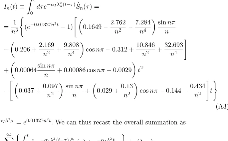
In(t)≡ Z t
0
dτ e−αIλ2n(t−τ)Sˆ
n(τ) =
= 1
n3 (
(e−0.01327n2t−1)
"
0.1649−2.762
n2 −
7.284 n4 sinnπ n −
0.206 + 2.169 n2 +
9.808 n4
cosnπ−0.312 +10.846 n2 +
32.693 n4
#
+
0.00064sinnπ
n + 0.00086 cosnπ−0.0029
t2
−
"
0.037 +0.097 n2
sinnπ n +
0.029 + 0.13 n2
cosnπ−0.144−0.434
n2 #
t
)
(A3)
sinceeαIλ2nτ =e0.01327n 2t
. We can thus recast the overall summation as
∞ X
n=1
Z t
0
dτ e−αIλ2n(t−τ)Sˆ
n(τ) +e−αIλ
2 ntc
n
sin (λnx)
= ∞ X
n=1 (
In(t) +
e−0.01327n2t n
0.73sinnπ
n −0.01 cosnπ−2.28
)
sinnπ L x ,
(A4)
which is clearly convergent, since everything is proportional to∝1/na.
The rst 30 terms in the summation att= 30sare plotted separately in Fig.A1; we see that only the rst six or seven matter signicantly. The largest contribution, for n= 1, is shown in Fig.A2, where the correction to the temperature (in absolute value) is maximal att= 0sand minimal at t∼50s.
The temperature prole inside the ice pad Eq.(54) is accordingly rewritten as follows,
u(x, t) = Tice(x, t) = [TI(t)−TS(t)]
x
L
+TS(t)
+ ∞ X n=1 Z t 0
dτ e−αIλ2n(t−τ)Sˆ
n(τ) +e−αIλ
2 ntc
n
sin (λnx)
= −(1.4×10⁻⁵t3−0.0012t2−0.0108t+ 4.1438)x L +2×10⁻⁵t3−0.0015t2−0.0065t−1.0633
+ ∞ X n=1 Z t 0
dτ e−αIλ2n(t−τ)Sˆ
n(τ) +e−αIλ
2 ntc
n
sin (λnx), (A5)
We remark that this result is specically valid for anyt≤60s, since the boundary conditionsTS(t)andTI(t) are interpolations corresponding only to such time interval.
Choosing dierent times will change the explicit form of both TS(t) and TI(t). On
the contrary, the temperature prole Eq.(54) found in Section 4 is given with implicit initial and boundary conditions, which makes it general and applicable to a range of diverse engineering problems.
References
Amirifard, F., Sharif, S. A., and Nasiri, F. (2018). Application of passive measures for energy conservation in buildings a review. Advances in Building Energy Research, 0(0), 134.
ASHRAE (1994). Refrigeration. Systems and Applications. Technical report, American Society of Heating, Refrigeration and Air-Conditioning Engineers.
ASHRAE (2010). Refrigeration. Systems and Applications. Technical report, American Society of Heating, Refrigeration and Air-Conditioning Engineers.
Bellache, O., Ouzzane, M., and Galanis, N. (2005). Numerical prediction of ventilation patterns and thermal processes in ice rinks. Building and Environment, 40(3), 417 426.
Bellache, O., Galanis, N., Ouzzane, M., Sunyé, R., and Giguère, D. (2006). Two-dimensional transient model of airow and heat transfer in ice rinks. ASHRAE Transactions, 112(2), 706 716.
Butera, F. M. (2013). Zero-energy buildings: the challenges. Advances in Building Energy Research, 7(1), 5165.
Caliskan, H. and Hepbasli, A. (2010). Energy and exergy analyses of ice rink buildings at varying reference temperatures. Energy and Buildings, 42(9), 1418 1425. Castellani, B., Gambelli, A., Morini, E., Nastasi, B., Presciutti, A., Filipponi, M.,
Nicolini, A., and Rossi, F. (2017). Experimental investigation on co2 methanation process for solar energy storage compared to co2-based methanol synthesis. Energies, 10(7), 855.
Castellani, B., Gambelli, A., Nicolini, A., and Rossi, F. (2019). Energy and environ-mental analysis of membrane-based ch4-co2 replacement processes in natural gas hydrates. Energies, 12(5), 850.
Chen, H., Zhang, X., Liu, J., and Tan, C. (2013). Compressed air energy storage. In Energy Storage-Technologies and Applications. IntechOpen.
Daoud, A., Galanis, N., and Bellache, O. (2008). Calculation of refrigeration loads by convection, radiation and condensation in ice rinks using a transient 3d zonal model. Applied Thermal Engineering, 28(1415), 1782 1790.
Erol, G. O., Açkkalp, E., and Hepbasli, A. (2017). Performance assessment of an ice rink refrigeration system through advanced exergoeconomic analysis method. Energy and Buildings, 138, 118 126.
European Parliament (2010). Directive 2010/31/EU of the european parliament and of the council of 19 may 2010 on the energy performance of buildings. Ocial Journal of the European Union 53 (2010) 13-35 .
Granryd, E. (2005). Refrigerating Engineering, Part II . KTH, Department of Energy Technology.
Haghighi, E. B., Makhnatch, P., and Rogstam, J. (2014). Energy saving potential with improved concrete in ice rink oor designs. International Journal of Civil, Environmental, Structural, Construction and Architectural Engineering, 8(6), 635 641.
Hahn, D. W. and Ozisik, M. N. (2012). Heat Conduction. John Wiley, 3rd edition. Hastaoglu, M. A., Negiz, A., and Heidemann, R. A. (1995). Three-dimensional
tran-sient heat transfer from a buried pipe Part III. Comprehensive model. Chemical Engineering Science, 50(16), 2545 2555.
Karampour, M. (2011). Measurement and modeling of ice rink heat loads. Master's thesis, Royal Institute Of Technology, Stockholm, Sweden.
Krarti, M. (1999). Building foundation heat transfer. BIOPROCESS TECHNOLOGY , 13, 241316.
Lu, T., Lü, X., Remes, M., and Viljanen, M. (2011). Investigation of air manage-ment and energy performance in a data center in Finland: Case study. Energy and Buildings, 43(12), 3360 3372.
Lü, X., Lu, T., Kibert, C. J., and Viljanen, M. (2014). A novel dynamic modeling approach for predicting building energy performance. Applied Energy, 114(0), 91 103.
Lü, X., Lu, T., Kibert, C. J., and Viljanen, M. (2015). Modeling and forecasting en-ergy consumption for heterogeneous buildings using a physicalstatistical approach. Applied Energy, 144(0), 261 275.
Mun, J. and Krarti, M. (2011). An ice rink oor thermal model suitable for whole-building energy simulation analysis. Building and Environment, 46(5), 1087 1093. Negiz, A., Hastaoglu, M. A., and Heidemann, R. A. (1993). Three-dimensional transient heat transfer from a buried pipe I. Laminar ow. Chemical Engineering Science, 48(20), 3507 3517.
Ohba, M. and Lun, I. (2010). Overview of natural cross-ventilation studies and the latest simulation design tools used in building ventilation-related research. Advances in Building Energy Research, 4(1), 127166.
Omri, M., Barrau, J., Moreau, S., and Galanis, N. (2016). Three-dimensional transient heat transfer and airow in an indoor ice rink with radiant heat sources. Building Simulation, 9(2), 175182.
Osram GmbH (2014). Osram POWERSTAR® HQI® - Technical Information. Tech-nical report, Osram.
Palmowska, A. and Lipska, B. (2018). Research on improving thermal and humidity conditions in a ventilated ice rink arena using a validated cfd model. International Journal of Refrigeration, 86, 373 387.
Poirier, L., Lozowski, E. P., and Thompson, R. I. (2011). Ice hardness in winter sports. Cold Regions Science and Technology, 67(3), 129 134.
Räikkönen, M. (2012). Jäähallin energiatehokkuus. Diploma thesis, Aalto University. Seghouani, L., Daoud, A., and Galanis, N. (2009). Prediction of yearly energy
require-ments of indoor ice rinks. Energy and Buildings, 41(5), 500 511.
Seghouani, L., Daoud, A., and Galanis, N. (2011). Yearly simulation of the interaction between an ice rink and its refrigeration system: A case study. International Journal of Refrigeration, 34(1), 383 389.
handling unit conguration eects on energy performance in an air-heated ice rink arena. Energies, 12(4).
Teyssedou, G., Zmeureanu, R., and Giguere, D. (2009). Thermal response of the con-crete slab of an indoor ice rink (RP-1289). Technical report, HVAC & R Research. Taylor & Francis Ltd.
Teyssedou, G., Zmeureanu, R., and Giguere, D. (2013). Benchmarking model for the ongoing commissioning of the refrigeration systemof an indoor ice rink. Automation in Construction, 35(0), 229 237.
Titchmarsh, E. (1962a). Eigenfunction Expansions part 1 . Oxford University Press (Clarendon Press).
Titchmarsh, E. (1962b). Eigenfunction Expansions part 2 . Oxford University Press (Clarendon Press).
Toomla, S., Lestinen, S., Kilpeläinen, S., Leppä, L., Kosonen, R., and Kurnitski, J. (2018). Experimental investigation of air distribution and ventilation eciency in an ice rink arena. International Journal of Ventilation, pages 117.
Tutumlu, H., Yumruta³, R., and Yildirim, M. (2018). Investigating thermal perfor-mance of an ice rink cooling system with an underground thermal storage tank. Energy Exploration & Exploitation, 36(2), 314334.
Yang, C., Demokritou, P., Chen, Q., Spengler, J., and Parsons, A. (2000). Ventilation and air quality in indoor ice skating arenas. ASHRAE Transactions, 106(2), 338 346.
Yang, C., Demokritou, P., Chen, Q., and Spengler, J. (2001). Experimental validation of a computational uid dynamics model for IAQ applications in ice rink arenas. Indoor Air, 11(2), 120126.
Figure 13. Temperature prole in the ice pad, analytical solution.
Figure 14. FEM solution fort= 0...60s.
Figure A1. Contribution of the rst 30 terms in the summation (A4), att= 30s.
Figure A2. Largest (n= 1) contribution, where 0< t <60s.