DOI: 10.1534/genetics.108.099556
Hierarchical Generalized Linear Models for Multiple
Quantitative Trait Locus Mapping
Nengjun Yi*
,1and Samprit Banerjee
†*Department of Biostatistics, Section on Statistical Genetics, University of Alabama, Birmingham, Alabama 35294 and†Divison of Biostatistics and Epidemiology, Department of Public Health, Weill Medical College of Cornell University, New York, New York 10021
Manuscript received December 9, 2008 Accepted for publication January 6, 2009
ABSTRACT
We develop hierarchical generalized linear models and computationally efficient algorithms for genomewide analysis of quantitative trait loci (QTL) for various types of phenotypes in experimental crosses. The proposed models can fit a large number of effects, including covariates, main effects of numerous loci, and gene–gene (epistasis) and gene–environment (G3E) interactions. The key to the approach is the use of continuous prior distribution on coefficients that favors sparseness in the fitted model and facilitates computation. We develop a fast expectation-maximization (EM) algorithm to fit models by estimating posterior modes of coefficients. We incorporate our algorithm into the iteratively weighted least squares for classical generalized linear models as implemented in the package R. We propose a model search strategy to build a parsimonious model. Our method takes advantage of the special correlation structure in QTL data. Simulation studies demonstrate reasonable power to detect true effects, while controlling the rate of false positives. We illustrate with three real data sets and compare our method to existing methods for multiple-QTL mapping. Our method has been implemented in our freely available package R/qtlbim (www.qtlbim.org), providing a valuable addition to our previous Markov chain Monte Carlo (MCMC) approach.
M
OST complex traits are influenced by interacting networks of multiple quantitative trait loci (QTL) and environmental factors (Carlborg and Haley2004). Mapping QTL is to infer which genomic loci are strongly associated with the complex trait and to estimate genetic effects of these loci,i.e., main effects and gene–gene (epistasis) and gene–environment (G3 E) interactions. Due to the multilocus nature of complex traits, it is desirable to simultaneously analyze multiple loci rather than one locus (or a few loci) at a time. How-ever, QTL mapping studies usually genotype hundreds or thousands of genomic loci (markers), leading to numerous variables and a huge number of possible mod-els, and the dependence of genotypes on a chromosome results in many correlated variables. Therefore, mapping multiple QTL requires sophisticated methods that can handle problems with high-dimensional correlated variables.
The popular approaches to mapping multiple QTL are some form of variable selection. Such techniques involve identifying a subset of all possible genetic effects (a multiple-QTL model) that best explains the pheno-typic variation. Classical variable selection methods use forward or stepwise search procedures and selection
criteria such as Bayesian information criteria (BIC) or modified versions to find a multiple-QTL model (Kao
et al.1999; Bromanand Speed2002; Bogdanet al.2004;
Baierlet al.2006). Bayesian methods proceed by setting
up a likelihood function for observed data and prior distributions on unobserved quantities. Two types of prior distributions have been suggested for multiple-QTL mapping. The first assumes a two-component mixture distribution for each genetic effect, typically a normal distribution with known or unknown variance and a point mass at zero. This discrete prior allows each effect to have positive probability of dropping out of the model (Yi2004; Yiand Shriner2008). The second formulation
takes continuous prior distributions for genetic effects that favor a sparse structure with many of the effects having values close to zero and few with large values (Meuwissen et al. 2001; Xu 2003; Yi and Xu 2008).
These Bayesian models are computed using Markov chain Monte Carlo (MCMC) algorithms to sample from the posterior distribution. Due to the recent develop-ment of MCMC algorithms and associated computer software, Bayesian methods have become increasingly popular in QTL mapping (Yiet al.2005, 2007a,b; Yandell
et al.2007; Yiand Shriner2008). The Bayesian MCMC
approaches can provide comprehensive information, but they are computationally intensive in interacting-QTL analysis. Further, the existing methods rely primar-ily upon normal linear models.
1Corresponding author: Department of Biostatistics, University of
Alabama, Birmingham, AL 35294-0022. E-mail: [email protected]
We present a unified methodology for mapping multiple QTL based upon the generalized linear model framework. The generalized linear model is the main tool for routine statistical analysis, enjoying a body of well-developed theory, algorithms, and software and includ-ing various models as special cases. However, classical generalized linear models cannot simultaneously han-dle many correlated variables. We propose a Bayesian generalized linear model approach, placing continuous prior distributions on genetic effects, to deal with the high-dimensional problem. Although various priors can be used for this purpose (Griffin and Brown 2007;
Parkand Casella2008), we consider the well-known
Student’st-distribution and recommend the choice of hyperparameters to yield a sharp mode at zero and to induce a sparse model. Our unified framework incor-porates the advantages of generalized linear models and hierarchical modeling into multiple-QTL mapping, allowing us to deal with various types of continuous and discrete phenotypes and to simultaneously analyze covariates, main effects of numerous loci, and epistatic andG3Einteractions.
In principle, we can fit our hierarchical generalized linear model by adapting the MCMC algorithms of Yi
and Xu (2008) for normal regressions. However, it is
desirable to have a quick calculation that estimates the posterior mode of genetic effects (a point estimate that maximizes the posterior distribution). Although the posterior mode estimate provides less information than a fully Bayesian MCMC analysis, such analyses are similar to classical QTL practice, are easy to understand, and can be valuable for identifying significant variables. Various methods have been proposed for the purpose, but they are built upon special models and optimiza-tion algorithms (Tibshirani 1996; Figueiredo 2003;
Kiiveri2003; Efronet al.2004; Genkinet al.2007) and
cannot be easily set up for multiple-QTL mapping. Re-cently, some mode-finding methods for mapping mul-tiple QTL have been suggested (Zhangand Xu2005;
Xu2007). However, these methods have dealt with only
continuous traits and have not been effectively imple-mented in computer software.
We present a fast expectation-maximization (EM) algorithm to fit our hierarchical generalized linear mod-els by estimating the posterior modes of coefficients. We develop our algorithm by making use of the two-level formulation of Student’st-density and expressing the prior information on coefficients as additional ‘‘data points.’’ This strategy allows us to incorporate our algorithm into the usual iteratively weighted least squares for general-ized linear models as implemented in R (R Development
Core Team 2006). This implementation takes
advan-tage of the well-developed existing algorithm and soft-ware, extending available tools for fitting generalized linear models to multiple-QTL mapping.
Although in principle our hierarchical model and algorithm can fit all possible effects in a single model, we
do not recommend this and rather propose a novel model search method to build a parsimonious model by seeking significant genetic effects. This procedure provides a flexible and convenient way to deal with large-scale QTL data and also has the advantage of accommo-dating the correlation structure in QTL data. Simulation studies demonstrate that our method provides reason-able power to detect true effects and can control the rate of extraneous effects. Real data analyses show that the proposed approach compares favorably to existing sophisticated methods.
METHODS
Generalized linear models of multiple QTL: We
consider experimental crosses derived from two inbred lines (for example, F2, backcross, and recombinant inbred lines). Observed data in QTL studies consist of pheno-typic values of a complex trait, genetic markers across the genome, and/or some relevant environmental fac-tors (covariates). The marker data include the geno-types and the genomic positions of markers. Mapping QTL is to identify genomic loci that associate with the phenotype and to estimate their genetic effects. For sim-plicity, we describe our methods by considering ob-served markers as potential QTL. The methods can be extended to consider loci between the observed markers. We use the generalized linear model framework to analyze various types of complex traits. A generalized linear model consists of three components: the linear predictor, the link function, and the distribution of the outcome variable (McCullagh and Nelder 1989;
Gelmanet al.2003). We simultaneously fit
environmen-tal effects, main effects of markers, epistatic effects, and gene–environment (G3E) interactions. Therefore, the linear predictor can be expressed as
h¼b01XEbE1XGbG1XGGbGG1XGEbGEbXb; ð1Þ
where b0 is the intercept, bE and bG represent the vectors of environmental effects and all possible main effects, respectively,bGG andbGE represent the vectors of all possible epistatic and G 3 E interactions, re-spectively, andXE,XG,XGG, andXGEare the correspond-ing design matrices of effect predictors. We describe the construction of these design matrices in the next section.
The invertible link function g relates the linear predictorhto the mean of the outcome variabley,
EðyjXÞ ¼g1ðhÞ ¼g1ðXbÞ; ð2Þ
where the vector y¼ ðy1;y2; ;ynÞ T
pðyjXb;fÞ ¼Y
n
i¼1
pðyijXib;fÞ; ð3Þ
where Xib¼hi is the linear predictor for the ith individual. Generalized linear modeling provides a unified framework for statistical analysis; by choosing appropriate link functions and data distributions, some commonly used models,e.g., normal linear (Gaussian), logistic, probit, and Poisson regressions, become special cases.
Construction of the design matrices: There is some
discussion in the QTL mapping literature on the best way to construct contrasts for genetic predictors (Zeng
et al.2005). Among those, due to its orthogonal
prop-erty, the Cockerham genetic model is widely used in QTL mapping and is applied in this study. For a back-cross design, the Cockerham model defines the values of the main-effect contrast as0.5 or 0.5 for two genotypes at any locus. For an intercross (F2) design, there are two types of main effects, called additive and dominance effects, and the original Cockerham model defines ad-ditive contrast as1, 0, and 1 for three genotypes and dominance contrast as0.5 and 0.5 for homozygotes and heterozygotes, respectively. To make additive and dominance contrasts have a common scale, however, we rescale additive contrast as20.5, 0, and 20.5. For loci
with missing genotypic values, we replace the values of the above contrasts by their conditional expectations given the observed marker data (Haley and Knott
1992). The conditional expectations can be calculated using the multipoint method ( Jiangand Zeng1997).
For each covariate, we transform the raw values to have a mean of 0 and a standard deviation of 0.5, by subtracting the mean and dividing by 2 3 SD (the standard deviation of the raw values) (Gelman et al.
2008). This transformation standardizes all the cova-riates to a common scale, the scale of all the genetic main effects described above. Finally, the epistatic contrastsXGGor theG3EcontrastsXGEare constructed by multiplying two corresponding main-effect contrasts.
Prior and posterior distributions: Mapping QTL is
equivalent to estimating coefficients b in the above model, including environmental effects, main effects of markers, and epistatic and G 3 E interactions. The number of coefficients in the model can be large and the predictors are highly correlated, precluding the use of classical maximum-likelihood methods. This problem could be solved by setting up a prior distribution onbto capture the notion that most of the components ofb are likely to be zero or at least negligible; such prior distributions are often referred to as shrinkage priors. For the intercept b0 and the dispersion parameter f if present, we use the uniform priors, pðb0Þ}1 and
pðfÞ}1.
We assume independent Student’s t-priors tnjð0;sj2Þ on coefficients bj, with nj andsj chosen to give each coefficient a high probability of being near zero while
still allowing for occasional large effects. We are moti-vated to use the t-distribution because it allows for robust inference, shrinkage estimation, and easy com-putation (Gelmanet al.2003). There is no easy way to
estimate the coefficients directly using the tdensities, but it is straightforward to deal with the two-level formulation of t distribution (Gelman et al. 2003,
2008). The t-distributiontnjð0;s 2
jÞcan be expressed as a mixture of normal distributions with mean 0 and variance distributed as scaled inverse-x2,
bjjt2jNð0;t2jÞ; t2j Invx2ðnj;sj2Þ; j ¼1; ;J;
ð4Þ
where J is the number of the coefficients, and the hyperparametersnj.0 andsj.0 represent the degrees of freedom and the scale of the distribution, respectively. The priors (4) introduce coefficient-specific varian-ces, resulting in distinct shrinkage for different coef-ficients. The variances tj are not the parameters of interest, but they are useful intermediate quantities to allow easy and efficient computation. The hyperpara-metersnj andsj affect the amount of shrinkage in the coefficient estimates and should be carefully chosen. We discuss our choice of nj and sj after describing our computational algorithm. Our algorithm highlights how these hyperparameters affect the estimates of the parameters.
With the above prior distributions, we can express the log-posterior distribution of the parameters (b;f;t2) as
logpðb;f;t2jy;XÞ
}X
n
i¼1
logpðyijXib;fÞ1
XJ
j¼1
logpðbjjt2jÞ
1 X
J
j¼1
logpðt2j jnj;sj2Þ}X
n
i¼1
logpðyijXib;fÞ
1
2 XJ
j¼1
logt2j 1b
2
j
t2j !
1 X
J
j¼1 nj
2logs 2
j
nj 2 11
logt2
j
njsj2
2t2j !
; ð5Þ
wheret2¼ ðt2
1; ;t2JÞ.
EM algorithm for computing the posterior mode:
Our hierarchical generalized linear model can be fit using MCMC algorithms, applied to the joint posterior distributionpðb;f;t2jy;XÞ(Gelmanet al.2003). How-ever, it is desirable to have a faster computation that estimates the posterior mode ofbandfby maximizing the marginal posteriorpðb;fjy;XÞrather than the full posterior distribution. The two-level hierarchical model described above allows us to obtain the posterior mode by using the EM algorithm (Gelmanet al.2003, 2008).
ap-proach built upon the standard algorithm for classical generalized linear models.
The analysis of classical generalized linear models uses iterative weighted linear regression to obtain approx-imate maximum-likelihood estapprox-imates for the parameters (as implemented in the R routine glm, for example). The basic method is to approximate the generalized linear model by a normal linear model and then apply the algorithm for normal linear models to estimate the parametersðb;fÞ(Gelmanet al.2003, 2008). At each
iteration, the algorithm proceeds by calculating pseu-dodatazi and pseudovariancess2i for each observation
ion the basis of the current estimates of the parameters
ðbˆ;fˆÞ, approximating the generalized likelihoodpðyij
Xib;fÞby the weighted normal likelihoodNðzijXib;s2iÞ, and then updating the parameters ðb;fÞ by weighted linear regression. The iteration proceeds until conver-gence. The pseudodatazi and pseudovariancess2i are calculated by
zi ¼hˆi
L9ðyijhˆi;fˆÞ L$ðyijhˆi;fˆÞ
; s2i ¼ 1
L$ðyijhˆi;fˆÞ
; ð6Þ
where ˆhi¼Xibˆ, Lðyijhˆi; fˆÞ ¼logpðyijXibˆ;fˆÞ, L9ðyij hi;fÞ ¼dLðyijhi;fÞ=dhi,L$ðyijhi;fÞ ¼d2Lðyijhi;fÞ=
dh2
i, and ˆband ˆfare the current estimates ofbandf, respectively.
Given the variances t2, the prior information on b [i.e.,bjjt2
j Nð0; t2jÞ] can be included in the classical generalized linear model asJadditional ‘‘observations’’ of value 0, with ‘‘predictor matrix’’ IJ and ‘‘residual variance matrix’’Sb¼diagðt21; ;t2JÞ, where IJ is the
J3Jidentity matrix (Gelmanet al.2003, 2008). Thus,
the generalized linear model with the normal prior onb can be approximated by
z*jX*;b;f NðX*b;S*Þ; ð7Þ
where
z*¼ z
0 ðn1JÞ31; X*¼
X IJ ðn1JÞ3J
; and S*¼ Sz 0
0 Sb
withSz¼diagðs2
1; ;s2nÞ. Thus, we can use the stan-dard iteratively weighted least-squares computation to estimateðb;fÞby performing a weighted regression of the augmented data vectorz* on the augmented pre-dictor matrix X* with augmented weight vector
w*¼ ðs12; ;s
2
n ;t
2
1 ; ;t
2
J Þ.
To implement the EM algorithm, we treat the un-known variances t2 ¼ ðt2
1; ;t 2
JÞ as missing data and average over them by replacing the terms involving both t2 and b in the joint posterior (5) by their expected values conditional on the current estimate of ðbˆ;fˆÞ. Thus, we must evaluate the conditional expectations of 1=t2
j for allj. It can be easily shown that the conditional posterior distribution of t2
j ¼ Invx 211n
j;ðnjs2j 1 ˆ
b2jÞ=ð11njÞ, and thus the conditional expectation of
1=t2 j ¼
ðnjsj21bˆ 2
jÞ=ð11njÞ 1
. Therefore, the E-step of our EM algorithm is equivalent to replacing the varian-ces by
ˆ t2j ¼njs
2
j 1bˆ
2
j
11nj ; j¼1; ;J; ð8Þ where ˆbjis the current estimate ofbj.
We have incorporated our algorithm into the stan-dard package glm in R for fitting generalized linear models. We altered the glm function by inserting the steps for calculating the augmented data (7) and updating the variances (8) into the iterative procedure in the glm function. Our algorithm is initialized by setting eachtjto a small value (saytj¼0.1) andðb;fÞto the starting value provided by the glm function. At each step of our algorithm, we average over the variancest2¼
ðt2
1; ;t2JÞand then update ðb;fÞby maximizing the posterior density (5). In summary, our algorithm pro-ceeds as follows:
1. On the basis of the current value ofðb;fÞ, calculate pseudodatazand pseudovariancess2 using (6). 2. E-step: replace each variance t2
j by its conditional expectation using (8).
3. M-step: perform the weighted least-squares regres-sion based on the augmented data to obtain the estimateðbˆ;fˆÞusing (7).
4. Repeat steps 1–3 until convergence.
We apply the criterion in the glm function to assess convergence. In practice our algorithm converges rapidly. At convergence of the algorithm, we obtain all the outputs produced by the glm function, including the latest estimate ˆb, their standard deviations and P -values (for testingbj ¼0), and some additional values (e.g., for the variances). The outputs are automatically stored as a standard glm object.
Choosing the hyperparameters: Before discussing
our choice of the hyperparametersnjandsjwe discuss the improper Jeffreys prior on the variances,pðt2
jÞ}t
2
j , which is equivalent to the uniform distribution on logt2 j and is the limiting case of the scaled inverse-x2 density with nj ¼0. The Jeffreys prior yields an improper posterior on eachbj with an infinite mode at zero. As
jbjj increases, however, a second finite local mode appears away from zero (e.g., ter Braak et al. 2005;
Griffin and Brown 2007). The property of a model
with the Jeffreys prior may make it problematic to fully explore the posterior, but still formally allows the analysis of posterior modes (see Griffin and Brown
2007). Much work has shown that the Jeffreys prior leads to good performance in MCMC and mode-finding analyses, yielding strong shrinkage for very small effects but weak shrinkage for large effects (Figueiredo2003;
Kiiveri2003; Xu2003; Baoand Mallick2004; Griffin
and Brown2007).
impropri-ety of both prior and posterior. This can be achieved by settingnjandsjto be small enough so that the variances ˆ
t2
j obtained by Equation 8 are close to zero for near-zero coefficients ( ˆb2j 0), but ˆb2j for large coefficients ( ˆb2j?njs2
j). We set nj ¼ 0.01 and sj ¼ 104 in our application. This prior works well and stably. However, we find that small changes from this default value (e.g., nj from 0 to 0.1, sj from 0 to 103) do not affect the results. The small positive value of nj and sj yields a proper prior on bj sharply peaked near zero but approximately uniform for the range away from zero and thus leads to strong sparseness in the fitted model while allowing for occasional large coefficients. Finally, our scaled inverse-x2prior includes uniform priors for bj as a special case (nj¼sj2¼‘), and thus we can perform no shrinkage for certain variables (e.g., relevant covariates).
Model search strategy:In principle the above
hierar-chical models can handle any number of variables [see the augmented regression (8), where the number of data points (n1J) is larger than the number of variables
J] and thus can simultaneously estimate genetic effects of a large number of markers. For biological interpret-ability, however, we prefer using only a subset of the genetic effects in the model. Furthermore, including all possible effects requires large memory and intensive computation. Therefore, we propose a model search strategy to build a parsimonious model, beginning with a model with no genetic effect but some relevant covariates if any, gradually adding different types of genetic effects into the model and then fitting the new model. It is expected that many variables have no effects on the phenotype and should be pruned from the model. We set a very small threshold valuet1(say 108) and delete genetic effects satisfyingjbˆjj,t1from the model.
Our approach differs from classical forward stepwise methods by simultaneously adding many correlated var-iables and deleting many near-zero varvar-iables. As de-scribed below, our search strategy can take advantage of the special correlation structure in QTL data: genotypes on the same chromosomes are correlated. In summary, our approach proceeds as follows:
1. Searching for main effects: for each chromosomec
(c¼1;2; ), simultaneously add all possible main effects for markers on chromosomecinto the current model, fit the model, and then delete some main effects on the basis of the above-mentioned criterion. 2. Searching for epistatic effects among the included main effects: simultaneously add all possible epistatic interactions among the included main effects into the current model, fit the model, and delete some epistatic effects.
3. Searching for epistatic effects between the excluded and the included main effects: for chromosome
c (c¼1;2; ), simultaneously add all possible epi-static interactions between the remaining main
effects (not included in the current model) on chromosome c and the included main effects into the current model, fit the model, and delete some epistatic effects added in this step.
4. Searching for interactions between the covariate(s) and main effects: for chromosome c (c¼1;2; ), simultaneously add all possible interactions between the covariate(s) and all possible main effects on chromosomecinto the current model, fit the model, and delete some G3 E interactions added in this step.
After these steps, we obtain a final model with preset covariates and genetic effects satisfying jbˆjj .t1. With our shrinkage prior, the majority of genetic effects are shrunk to zero, and thus the final model includes only a limited number of variables. As shown in our simulation studies, our model search procedure picks up true effects with reasonable high probability, but can occa-sionally include some extraneous effects. However, inclusion of spurious effects has little effect on detecting and estimating true or strong effects, and the estimates of spurious effects (and the correspondingP-values) are smaller (larger) than those of the true effects, allowing us to easily identify strong causal effects. Although not necessary, however, it could be useful to have a formal procedure to remove extraneous effects from the final model. A simple way is to use the P-values for testing bj¼0 (equivalent to the likelihood-ratio test) in the final model; we set a small threshold valuet2(say 0.001) and remove genetic effects with theP-values larger than
t2from the model. As described later, a value of t2¼ 0.001 can greatly reduce the rate of false positives. However, the P-values should be interpreted with caution, as they are based on the final model.
Implementation in R/qtlbim: The freely available
package R/qtlbim (www.qtlbim.org) is an extensible and interactive environment for multiple-QTL mapping in experimental crosses (Yandellet al.2007), built on top
of the widely used R/qtl (Bromanet al.2003). The
pre-vious version of R/qtlbim performs fully Bayesian analyses via MCMC algorithms to simultaneously handle covariates, main effects, epistatic and gene–environment interactions for continuous traits, and binary and ordinal traits. We have incorporated the proposed method into R/qtlbim, by creating new functions to implement our model-fitting algorithm and model search procedure. The outputs for the final model are stored as a standard glm object and thus can be summarized and displayed conventionally.
SIMULATION STUDIES
Simulation design:Although our method can handle
basic conclusions hold for other cases. In our simula-tions, we generated the continuous phenotypes on the basis of different multiple-QTL models and the binary trait by transforming the continuous values into two categories with the proportions of 40 and 60%, re-spectively. We generated a genome with 19 chromo-somes, each of length 100 cM. Five percent of the marker genotypes were assumed to be randomly missing.
The first experiment was an F2intercross composed of 400 progenies and having 11 equally spaced markers (placed 10 cM apart) on each chromosome. We consid-ered a model with one binary covariate and five QTL with only main effects. The covariate effect explained
4% of the variance of the continuous phenotype. Table 1 presents the simulated positions of five QTL, their additive or dominance effects, and the approximate her-itabilities (proportion of the phenotypic variation ex-plained by an effect). As can be seen, two of five simulated QTL (Q2 and Q4) were positioned at markers, and others were in marker intervals. The second simulation was the same as the first one except that each chromo-some had 51 equally spaced markers (placed 2 cM apart). Therefore, these two simulations had 209 and 969 total markers, respectively.
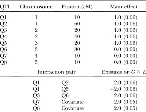
Our third experiment was a backcross (BC) with 400 progenies and 11 equally spaced markers on each chro-mosome. We simulated one binary covariate and eight QTL with complex interactions; among the eight simulated QTL, five had main effects while other three had no main effects but interacted with other QTL or the covariate. The covariate effect explained2% of the variance of the continuous phenotype. Table 2 presents the positions of simulated QTL, the genetic effects (main effects, epistasis, andG3 E), and the approxi-mate heritabilities. The fourth simulation was the same as the third except that each chromosome had 51 equally spaced markers.
Analysis and evaluation: Under each scenario, we
carried out 200 simulation replicates. Each of the F2 simulated data sets was analyzed using two models; the first included a covariate term and main effects of all markers, and the second allowed not only the covariate and main effects but also epistatic andG 3E interac-tions. The aim of the second analysis is to examine
whether or not we detect interactions if they are not present. For each of the simulated backcross (BC) data sets, we fit a model with a covariate effect, main effects of all markers, and epistatic andG3Einteractions. For all analyses, the continuous and the binary traits were analyzed using Gaussian and Probit models, respectively. We tried several values for the hyperparameters nj from 0 to 0.1 andsjfrom 0 to 103and got similar results. We displayed the results with (nj,sj)¼(0.01, 104). To investigate the influence of two thresholdst1andt2on our model search method (see the last section), we analyzed the data sets using several values (t1¼ 104, 106, 108, 1010, 1012, andt
2¼1, 0.01, 0.005, 0.001). We evaluated the performance of our method by examining the frequency of each effect included in the final model, true positives (the frequency of true effects included in the final model), and false positives (the frequency of false effects included in the final model) over the 200 simulation replicates. The inclusion frequency of an effect presents the empirical power to detect the effect. A detected main or G 3 E effect (epistatic effect) is considered as correct if the associated position(s) is within 10 cM of any true QTL.
Results:The thresholdt1controls the minimal size of
genetic effects to enter the models. We found that the final models almost picked up the same sets of effects for the above values oft1in all the simulation experiments, and thus the choice of t1 had little influence on our model search method. Therefore, we present only the results fort1¼108below.
Figure 1 displays the genetic effects included in the final models with frequencies.0.01 for the four values oft2in the first simulation experiment. We can see that no false effect (defined above) was included the final models with frequency.0.01. For the continuous trait, the simulated main effects located at markers, (1@60)d
TABLE 1
F2simulation with five main-effect QTL
QTL Chromosome Position (cM) Main effect
Q1 1 12 a¼0.5 (0.08)
Q2 1 60 d¼0.7 (0.08)
Q3 2 23 a¼ 0.5 (0.08)
Q4 2 50 a¼0.5 (0.08)
Q5 8 24 a¼0.4 (0.05)
d¼ 0.5 (0.04)
The effectsaanddrepresent additive and dominance ef-fects, respectively.
TABLE 2
Backcross simulation with eight interacting QTL
QTL Chromosome Position(cM) Main effect
Q1 1 10 1.0 (0.06)
Q2 1 60 1.0 (0.06)
Q3 2 20 1.0 (0.06)
Q4 2 40 1.0 (0.06)
Q5 3 20 1.0 (0.06)
Q6 3 80 0.0 (0.00)
Q7 4 10 0.0 (0.00)
Q8 5 10 0.0 (0.00)
Interaction pair Epistasis orG3E
Q1 Q2 2.0 (0.06)
Q1 Q5 2.0 (0.06)
Q3 Q6 2.0 (0.06)
Q7 Covariate 2.0 (0.05) Q8 Covariate 2.0 (0.05)
and (2@50)a, were detected with frequencies close to 1. As expected, the analyses of the binary trait had lower power than the continuous trait, especially for the two linked QTL on chromosome 2. For the simulated effects located within the marker intervals, our analyses picked up the corresponding effects of the flanking markers in the final models; for example, for the simulated effect (2@23)a, the final models included (2@20)aor (2@30)a. For these simulated effects, the true positives that roughly equal the sum of the inclusion frequencies of the corresponding flanking marker effects were also high. Although no interactions were present, the anal-yses allowing epistatic andG3Eeffects did not reduce the power for detecting the main effects and did not include any interactions with high frequency. Finally, it can be seen that a smaller thresholdt2slightly reduced
the power. However, this threshold controls the rate of false positives, which will be illustrated shortly.
Figure 2 shows the results of the analyses for the second experiment. The models including or excluding epistatic andG3Einteractions produced similar results again. Our second experiment simulated 51 markers evenly distributed on each chromosome, resulting in much higher correlation among the variables. Conse-quently, the simulated effects were included with lower frequencies than in the first experiment. However, we were still able to identify the true effects with reasonable high power and true positives for both the continuous and the binary traits. For example, the first simulated effect (1@12)a was identified with power of 60% (40%) and true positives of 90% (80%) for the con-tinuous (binary) trait.
Figure 1.—F
2 simulation with 19 chromosomes each having 100 cM and 11 markers: frequen-cies of effects included in final models over 200 replicates with the thresholds t1 ¼ 108 and t2¼1, 0.01, 0.005, and 0.001 for the continuous trait (circles) and the binary trait (triangles). Effects with frequencies ,0.01 are not displayed. The right (left) panel represents analyses exclud-ing (includexclud-ing) epistatic andG3 E interactions. The notation for effects, e.g., (1@10)a, indicates chromosome 1, position 10 cM, and additive effect a (or domi-nance effectd).
Figure 2.—F2 simulation with
The results for the BC simulations are illustrated in Figure 3. For the experiment with 11 markers on each chromosome, no false effect was included the final models with frequency.0.01. For the continuous trait, all the simulated main effects and epistatic andG3 E
interactions were identified in almost all 200 replicates. For all the simulated main effects and epistatic inter-actions, the analyses of the binary trait had lower power; the reduction of the power was larger for the main effects of the two relatively tightly linked QTL on chromosome 2 and epistasis. For the fourth experiment where 51 markers were evenly placed on each chromo-some, most of the simulated effects were included in the final models with frequencies.60% for the continuous
trait. Higher correlation among the variables resulted in the method occasionally picking up effects with associ-ated positions near to the true effects. Again, the true positives for all the simulated effects were high. Finally, it was observed that the thresholdt2had little influence on the power of detecting the true effects.
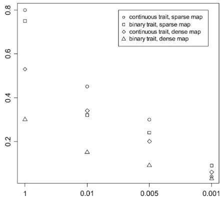
Figure 4 shows the false positives for the BC experi-ments under different P-values t2. The other experi-ments gave similar results. With a large value t2, the models included extraneous effects with high frequen-cies in the simulation replicates. Data with dense marker maps generally produced lower false positives. False effects were removed from the models rapidly as the thresholdt2decreased, indicating that false effects were associated with larger P-values. For all the cases, we observed that the estimates of the simulated effects were close to the corresponding true values. But the estimates of spurious effects were much smaller.
REAL DATA EXAMPLES
We illustrate our method with three real QTL mapping experiments. These data sets have been extensively analyzed previously and thus serve as good examples to compare our method with the existing methods and to illustrate the advantages of our method in terms of statistical and computational efficiencies and modeling flexibility. We used several values for nj (between 0 and 0.1) and sj (between 0 and 103) and obtained identical results. We displayed the results by setting the thresholdst1¼108andt2¼1.
Barley data set: The barley data set (Tinkeret al.
1996) was reanalyzed for demonstration. The data were collected from a doubled-haploid population that con-tained n ¼145 lines; each was grown in 25 different environments. The phenotype analyzed was the average value of kernel weight across environments. A total of Figure 3.—Backcross
simula-tion with 19 chromosomes each having 100 cM and 11 (right) or 51 (left) markers: frequencies of effects included in final models over 200 replicates with the thresholdst1¼ 108 and t2¼ 1, 0.01, 0.005, and 0.001 for the con-tinuous trait (circles) and the bi-nary trait (triangles). Effects with frequencies ,0.01 are not displayed. The notation for ef-fects,e.g., (1@10), indicates chro-mosome 1 and position 10 cM. The term fix.cov represents the covariate, and X1:X2 represents interaction between X1and X2.
Figure 4.—False positive rates for the threshold t2 ¼ 1,
127 markers spanning seven chromosomes were geno-typed. The data contained 5% missing marker genotypes.
We used a Gaussian model to fit main effects of all markers and their epistatic interactions. The total num-ber of effects was 8129 (127 main effects and 1273126/ 2¼8001 epistatic effects). Our analysis took0.05 min on a P4 computer. We obtained a final model with 8 main effects: 3 on chromosome 1; 2 on chromosome 2; and 1 on chromosomes 3, 4 and 7, respectively. We did not detect epistatic effects. The estimates of the main effects are displayed in the top panel of Figure 5. TheP -values for these effects were 1.3e-07, 3.3e-15, 1.4e-03, 4.3e -05, 6.9e-04, 9.2e-05, 3.3e-03, and 3.1e-24, respectively. If we sett2¼0.001, the effects [email protected] and [email protected] are removed from the final model. For comparison, we reanalyzed the data using the MCMC method (Yiet al.
2005, 2007a) implemented in R/qtlbim (Yandellet al.
2007). Our MCMC analysis also did not detect epistatic effects, but did detect multiple main effects with positions overlapping or close to those in the proposed method analysis (see the bottom panel of Figure 5).
This data set has been extensively analyzed using different methods, including mode-finding algorithms (Xu 2007; Xu and Jia 2007) and shrinkage MCMC
methods (Xu2003; Yiand Xu2008). Xu(2007) (also see
Xu and Jia 2007) analyzed this data set using an
empirical Bayes method and the LASSO of Tibshirani
(1996). Both the analyses took 2 min and obtained results similar to ours. The shrinkage MCMC algorithms also gave similar results, but took a few hours (Xu2003;
Yiand Xu2008). Therefore, our method performs
com-parably to the alternative sophisticated techniques and is computationally faster.
Listeria monocytogenes data set: As a second study we
illustrate the application of our method by reanalyses of the mouse data of Boyartchuket al.(2001). This data
set consisted of 116 female mice from an intercross (F2) between the BALB/cByJ and C57BL/6ByJ strains. Each animal was genotyped at 133 markers spanning 20 chromosomes. The phenotype of interest was the time to death following infection withL. monocytogenes. The animals that died from infection had a mean survival of 153.8 hr. Roughly 30% of the mice recovered from the infection and survived past the 264-hr time point. Sev-eral methods have been applied to this data set, in-cluding a two-part model (Broman2003), a parametric
proportional hazards model (Diao et al. 2004) and a
unified semiparametric framework approach ( Jinet al.
2007). These analyses detected significant QTL on chro-mosomes 1, 5, and 13 and suggestive QTL on chromo-some 15.
We applied our method to the data using the two-part model of Broman(2003) rather than developing a new
model for this type of phenotype. The two-part model decomposes the phenotype into a binary trait, indicat-ing whether the subject survived, and a continuous trait for time to death for those dying within 264 hr (Broman
2003). We used a Probit regression model for the binary phenotype and a Gaussian model for the logarithm of the continuous phenotype, and fit a model with main effects of all markers and their epistatic interactions. The total number of effects was 35,378 (133 additive effects, 133 dominance effects, and 35,112 epistatic effects).
Our analyses took0.02 and 0.03 min on a P4 com-puter, for the continuous and the binary traits, respec-tively. Our results were consistent with the previous ones Figure5.—Barley data set analyses using the
(Figure 6). For the continuous trait, the final model included two additive effects on chromosomes 1 and 15, respectively, and one dominance effect on chromosome 13. TheP-values for these effects were 3.8e-05, 1.8e-02, and 1.6e-03, respectively. For the binary trait, the final model included two additive effects on chromosomes 5 and 13, with the P-values being 1.7e-07 and 1.9e-04, respectively. We did not detect epistatic effects.
We also analyzed the data using the Bayesian MCMC method (Yiet al.2005, 2007a,b; Yandellet al.2007). The
MCMC algorithm detected additive effects on chromo-somes 1 and 15 and a dominance effect on chromosome 13 for the continuous trait and additive effects on chromosomes 5 and 13 for the binary trait (not shown here). The positions of these QTL were close to the markers detected by the proposed method. In addition these main effects, the fully Bayesian analysis found evidence of epistatic effects: for the continuous trait, QTL on chromosomes 1, 5, and 9 showed evidence of epistasis, and for the binary trait, chromosomes 6 and 13 harbored epistatic QTL. However, these epistatic effects were not strong. The MCMC analyses took 8 and 10 min for the continuous and the binary traits, respectively.
Obesity data set: We also applied our method to an
obesity data set of backcross mice. This data set has been extensively analyzed using Bayesian MCMC methods (Yi
et al.2005, 2006, 2007a). The cross was produced from
two highly divergent strains: M16i, consisting of large and moderately obese mice, and CAST/Ei, a wild strain of small mice with lean bodies. CAST/Ei males were mated to M16i females, and F1males were backcrossed to M16i females, resulting in 421 mice (213 males and 208 females) reaching 12 weeks of age. All mice were
genotyped for 92 markers located on 19 autosomal chromosomes. We analyzed a continuous trait Fat, the sum of right gonadal and hindlimb subcutaneous fat pads. We included sex and body weight at the age of 12 weeks as covariates and permitted the inclusion of epistatic and gene–sex interactions in a Gaussian re-gression model. The total number of genetic effects was 4370, including 92 main effects, 4186 epistatic effects, and 92 gene–sex interactions.
Using the MCMC algorithm (which took15 min), Yi
et al. (2007a) detected evidence of QTL on nine
chromosomes (1, 2, 6, 8, 13, 14, 15, 18, and 19). These QTL showed a complex network of interactions. The strongest main-effect QTL was found on chromosome 2, and QTL on chromosomes 8, 13, 14, 15, and 19 also had main effects. Strong epistatic interactions between chromosomes 15 and 19 and chromosomes 1 and 18 were detected. Evidence of epistasis was found between a few other chromosome pairs. The QTL on chromo-some 2 was found to interact with the covariate sex.
Our hierarchical generalized linear model analysis took0.15 min and obtained a final model including 12 main effects, 5 epistatic effects, and two gene–sex inter-actions. The estimates of the genetic effects and their
P-values are displayed in Figure 7. Our results were basi-cally consistent with the previous full Bayesian analysis; all strong effects were detected by both analyses. All the main-effect QTL detected in Yiet al.(2007a) were also
identified in our reanalysis, with positions in the regions detected previously. TheP-values for most of the main effects were,0.001. Main effects of two linked markers on chromosome 2 were simultaneously included in the model, which were the largest among the detected main effects. The epistatic interactions (19@38):(15@39) and Figure6.—Listeria monocytogenesdata set
(1@55):(18@73) were the strongest, which were also detected previously. Main effects on both chromosomes 1 and 18 were not included in the final model, indicating that our method can detect QTL with weak main effects but strong epistasis. Two gene–sex interactions, (2@73): SEX and (15@12):SEX, were included in the final model withP-values being 1.7e-03 and 4.4e-03, respectively.
DISCUSSION
We propose a new statistical framework for genome-wide multiple QTL mapping in experimental crosses. Our method is developed on the basis of the generalized linear model framework and thus can deal with various phenotypes that the standard generalized linear models can analyze. The proposed models assume sparseness-inducing priors and thus can simultaneously fit a large number of effects, including environmental effects, main effects of numerous genomic loci, and epistatic andG3Einteractions. By looking for the modes of the posterior distribution via the EM algorithm we are able to quickly identify significant effects. Experiments with extensive simulation studies and real data sets have shown good performance.
We assign independent normal distributions with unknown variances to the coefficients and devote our attention to the scaled inverse-x2 distribution for the variance parameters. Our prior includes the noninfor-mative Jeffreys prior as a special case, which has the form of a scaled inverse-x2density with 0 d.f. As already shown in previous studies (Figueiredo2003; Kiiveri2003; Xu
2003; Bao and Mallick 2004; Griffin and Brown
2007) and in our experimental results, the Jeffreys prior usually yields good performance, inducing strong spars-eness in the fitted model. However, we recommend choosing the hyperparameters in the scaled inverse-x2 to yield a proper prior on coefficients sharply peaked near zero but approximately uniform for the range away from zero. Our prior induces strong shrinkage for near-zero effects but weak shrinkage for large effects. Our method can be in principle extended to models with other prior distributions, for example, the exponential distributions with fixed hyperparameters. However, it would be appealing to treat the hyperparameters as unknowns and estimate them from the data so that the model can shrink the coefficients as much as can be justified by the data. Yi and Xu (2008) developed
MCMC algorithms to jointly estimate all hyperpara-meters and model parahyperpara-meters and found that such procedures usually outperform those with fixed hyper-parameters. Future research will extend the proposed EM algorithm to estimate hyperparameters.
Gelmanet al.(2008) proposed independent Cauchy
distribution with mean 0 and scale 2.5 [i.e., bjjt2 j
Nðmj;t2
jÞandt2j Inv-x2ð1;2:5Þ] for routine data anal-ysis, and implemented a procedure to fit generalized linear models with this prior by incorporating an EM algorithm into the usual iteratively weighted least squares. However, this Cauchy prior cannot shrink small effects to zero and thus cannot be used for our high-dimensional models. Our algorithm is similar to that of Gelman et al.(2008), but differs in regarding the
var-iances rather than the coefficients as missing data. The trick of the algorithm is to express the prior information Figure7.—Obesity data set analysis. The
on coefficients as additional ‘‘data points,’’ allowing us to take advantage of the existing iteratively weighted least-squares algorithm. Various other efficient methods have been proposed recently, but are built upon special algorithms and thus more difficult to implement (e.g., Tibshirani1996; Efronet al.2004; Genkinet al.2007;
Xu2007).
Rather than fitting all possible effects in a large model, we propose a novel model search strategy to build a parsimonious model. Our method begins with a model with no genetic effect and then adds different types of genetic effects into the model and deletes very small effects. Unlike the traditional variable selection ap-proach, we simultaneously add or delete many variables and take care of the correlation among the variables. Kiiveri (2003) and Zhangand Xu (2005) adopted a
similar criterion for pruning effects from the model, but used a backward selection procedure. Our search strategy avoids the need of large memory and compu-tational problems when the number of effects is huge, and thus facilitates the genomewide interacting QTL analysis.
The fully Bayesian approach, employing the MCMC simulation to generate posterior samples from the joint posterior distribution of all unknowns, can provide more comprehensive posterior inferences (Gelmanet al.2003).
In QTL mapping, the fully Bayesian methods can easily treat missing genotypes and positions of QTL as un-knowns and use model averaging to induce robustness and stability (Yiet al. 2005, 2007a,b; Yi and Shriner
2008). We describe our method by allowing only ob-served markers as potential QTL and replacing missing marker genotypes by their conditional expectations. We can extend our method to detect QTL within marker intervals by inserting loci within each marker interval (pseudomarkers) as possible positions of QTL. Further investigation may be needed on how the number and the spacing of pseudomarkers affect the performance of the method. The proposed method has computational advantages over the fully Bayesian MCMC methods. High-order interactions could be implemented using our approach, but this would substantially increase the model space to be explored and thus may need further investigation. Future research will extend our method to genomewide association analysis and gene expression QTL (eQTL) mapping. Fast and efficient algorithms are an essential feature for the practical analysis of these more complicated cases.
This work was supported by National Institutes of Health grant R01 GM069430 to N.Y. and partially supported by Clinical and Trans-lational Sciences Center grant UL1-RR024996 to S.B.
LITERATURE CITED
Baierl, A., M. Bogdan, F. Frommletand A. Futschik, 2006 On
lo-cating multiple interacting quantitative trait loci in intercross de-signs. Genetics173:1693–1703.
Bao, K., and B. K. Mallick, 2004 Gene selection using a two-level
hierarchical Bayesian model. Bioinformatics20:3423–3430. Bogdan, M., J. K. Ghoshand R. W. Doerge, 2004 Modifying the
Schwarz Bayesian information criterion to locate multiple inter-acting quantitative trait loci. Genetics167:989–999.
Boyartchuk, V. L., K. W. Broman, R. E. Mosher, S. E. F. D’Orazio,
M. N. Starnbach et al., 2001 Multigenic control of Listeria
monocytogenessusceptibility in mice. Nat. Genet.27:259–260. Broman, K. W., 2003 Mapping quantitative trait loci in the case of a
spike in the phenotype distribution. Genetics163:1169–1175. Broman, K. W., and T. P. Speed, 2002 A model selection approach
for identification of quantitative trait loci in experimental crosses. J. R. Stat. Soc. B64:641–656.
Broman, K. W., H. Wu,S´. Senand G. A. Churchill, 2003 R/qtl:
QTL mapping in experimental crosses. Bioinformatics 19:
889–890.
Carlborg,O¨., and C. Haley, 2004 Epistasis: too often neglected in
complex trait studies? Nat. Rev. Genet.5:618–625.
Diao, G., D. Y. Linand F. Zou, 2004 Mapping quantitative trait loci
with censored observations. Genetics168:1689–1698.
Efron, B., T. Hastie, I. Johnstoneand R. Tibshirani, 2004 Least
angle regression. Ann. Stat.32:407–499.
Figueiredo, M. A. T., 2003 Adaptive sparseness for supervised
learn-ing. IEEE Trans. Patt. Anal. Mach. Intell.25:1150–1159. Gelman, A., J. Carlin, H. Sternand D. Rubin, 2003 Bayesian Data
Analysis.Chapman & Hall, London.
Gelman, A., A. Jakulin, M. G. Pittauand Y. S. Su, 2008 A weakly
informative default prior distribution for logistic and other re-gression models. Ann. Appl. Stat. (in press).
Genkin, A., D. D. Lewisand D. Madigan, 2007 Large-scale
Bayes-ian logistic regression for text categorization. Technometrics49:
291–304.
Griffin, J. E., and P. J. Brown, 2007 Bayesian adaptive lassos with
non-convex penalization. Technical Report, University of War-wick, Coventry, UK.
Haley, C. S., and S. A. Knott, 1992 A simple regression method for
mapping quantitative trait loci in line crosses using flanking markers. Heredity69:315–324.
Jiang, C., and Z.-B. Zeng, 1997 Mapping quantitative trait loci with
dominant and missing markers in various crosses from two in-bred lines. Genetica101:47–58.
Jin, C., J. P. Fineand B. S. Yandell, 2007 A unified semiparametric
framework for quantitative trait loci analysis, with application to spike phenotypes. J. Am. Stat. Assoc.102:56–67.
Kao, C. H., Z-B. Zengand R. D. Teasdale, 1999 Multiple interval
mapping for quantitative trait loci. Genetics152:1203–1216. Kiiveri, H., 2003 A Bayesian approach to variable selection when
the number of variables is very large, pp. 127–143 in Science and Statistics: Festschrift for Terry Speed(Institute of Mathematical Statistics Lecture Notes—Monograph Series, Vol 40), edited by D. R. Goldstein. Hayward, CA.
McCullagh, P., and J. A. Nelder, 1989 Generalized Linear Models,
Ed. 2. Chapman & Hall, London.
Meuwissen, T. H. E., B. J. Hayes and M. E. Goddard,
2001 Prediction of total genetic value using genome-wide dense marker maps. Genetics157:1819–1829.
Park, T., and G. Casella, 2008 The Bayesian Lasso. J. Am. Stat.
Assoc.103:681–686.
R DevelopmentCoreTeam, 2006 R: A Language and Environment for
Statistical Computing. R Foundation for Statistical Computing, Vienna. http://www.R-project.org.
terBraak, C., M. Boerand M. Bink, 2005 Extending Xu’s Bayesian
model for estimating polygenic effects using markers of the en-tire genome. Genetics170:1435–1438.
Tibshirani, R., 1996 Regression shrinkage and selection via the
Lasso. J. R. Stat. Soc. B58:267–288.
Tinker, N. A., D. E. Mather, B. G. Rossnagel, K. J. Kashaand
A. Kleinhofs, 1996 Regions of the genome that affect
agro-nomic performance in two-row barley. Crop Sci.36:1053–1062. Xu, S., 2003 Estimating polygenic effects using markers of the entire
genome. Genetics163:789–801.
Xu, S., 2007 An empirical Bayes method for estimating epistatic
ef-fects of quantitative trait loci. Biometrics63:513–521. Xu, S., and Z. Jia, 2007 Genome-wide analysis of epistatic effects for
Yandell, B. S., T. Mehta, S. Banerjee, D. Shriner, R. Venkataraman
et al., 2007 R/qtlbim: QTL with Bayesian interval mapping in ex-perimental crosses. Bioinformatics23:641–643.
Yi, N., 2004 A unified Markov chain Monte Carlo framework for
mapping multiple quantitative trait loci. Genetics167:967–975. Yi, N., and D. Shriner, 2008 Advances in Bayesian multiple QTL
mapping in experimental designs. Heredity100:240–252. Yi, N., and S. Xu, 2008 Bayesian LASSO for quantitative trait loci
mapping. Genetics179:1045–1055.
Yi, N., B. S. Yandell, G. A. Churchill, D. B. Allison, E. J. Eisenet al.,
2005 Bayesian model selection for genome-wide epistatic QTL analysis. Genetics170:1333–1344.
Yi, N., D. K. Zinniel, K. Kim, E. J. Eisen, A. Bartolucci et al.,
2006 Bayesian analysis of multiple epistatic QTL models for body weight and body composition in mice. Genet. Res.87:45–60.
Yi, N., D. Shriner, S. Banerjee, T. Mehta, D. Pompet al., 2007a An
efficient Bayesian model selection approach for interacting QTL models with many effects. Genetics176:1865–1877.
Yi, N., S. Banerjee, D. Pompand B. S. Yandell, 2007b Bayesian
mapping of genome-wide interacting QTL for ordinal traits. Ge-netics176:1855–1864.
Zeng, Z.-B., T. Wangand W. Zou, 2005 Modeling quantitative trait
loci and interpretation of models. Genetics169:1711–1725. Zhang, Y.-M., and S. Xu, 2005 A penalized maximum likelihood
method for estimating epistatic effects of QTL. Heredity 95:
96–104.