Bayesian Inference of Recent Migration Rates Using Multilocus Genotypes
Gregory A. Wilson and Bruce Rannala
1Department of Medical Genetics, University of Alberta, Edmonton, Alberta T6G 2H7, Canada Manuscript received May 22, 2002
Accepted for publication December 10, 2002
ABSTRACT
A new Bayesian method that uses individual multilocus genotypes to estimate rates of recent immigration (over the last several generations) among populations is presented. The method also estimates the posterior probability distributions of individual immigrant ancestries, population allele frequencies, population inbreeding coefficients, and other parameters of potential interest. The method is implemented in a computer program that relies on Markov chain Monte Carlo techniques to carry out the estimation of posterior probabilities. The program can be used with allozyme, microsatellite, RFLP, SNP, and other kinds of genotype data. We relax several assumptions of early methods for detecting recent immigrants, using genotype data; most significantly, we allow genotype frequencies to deviate from Hardy-Weinberg equilibrium proportions within populations. The program is demonstrated by applying it to two recently published microsatellite data sets for populations of the plant speciesCentaurea corymbosaand the gray wolf speciesCanis lupus. A computer simulation study suggests that the program can provide highly accurate estimates of migration rates and individual migrant ancestries, given sufficient genetic differentiation among populations and sufficient numbers of marker loci.
I
N recent decades, indirect estimates of gene flow 1999, 2001;VitalisandCouvet2001). However, even coalescent-based methods currently assume that popula-(reviewed inSlatkinandBarton1989) have beenwidely used by biologists, first with allozyme data and tion demography has followed a relatively simple model of either constant size or deterministic expansion (with more recently with restriction fragment length
polymor-phisms (RFLPs), DNA sequence data, microsatellite constant migration rates) for roughly the last 4Ne gener-ations, which is the average time until the sampled chro-markers, and single-nucleotide polymorphisms (SNPs).
Direct estimates of migration rates based on mark-recap- mosomes coalesce to a most recent common ancestor (Kingman1982). For populations with largeNeor spe-ture or other methods can be impractical for large
popu-cies in highly disturbed habitats, this assumption may lations that exchange small numbers of migrants
be-be unreasonable. cause the expected number of recaptures is too low;
Recently, nonequilibrium approaches have been pro-indirect estimates of gene flow using genetic markers
posed for identifying migrants (Rannala and
Moun-are often the only recourse. Commonly used indirect
tain1997;Pritchardet al. 2000) or hybrids between estimators of gene flow, such as 4Nem⫽1/FST⫺1, are
species (AndersonandThompson2002) and assigning derived on the basis of simplified models of population
individuals of unknown population affinity to potential structure that assume constant population sizes,
sym-source populations using multilocus genotypes (
Paet-metrical migration (at constant rates), and population
kauet al. 1995;RannalaandMountain1997;Cornuet
persistence for periods sufficient to achieve genetic
et al. 1999;DawsonandBelkhir2001;Gaggiottiet al.
equilibrium (Wright1931, 1969).
2002). These methods extract information about recent The development of coalescent theory (Kingman1982;
migration (within the last few generations) from tran-reviewed byTavare 1984), which traces the ancestral
sient disequilibrium observed at individual multilocus genealogy of a sample rather than modeling changes
genotypes of migrants or individuals recently descended of gene frequencies in the population as a whole, has
from migrants. In comparison with indirect estimators allowed less restrictive models to be used in developing
of long-term gene flow, these methods make relatively indirect estimators of gene flow. The new methods
ac-few assumptions, but are informative only about recent commodate recent population expansions,
nonsymmet-patterns of migration. The two approaches (long-term rical migration, and other complexities that are typical
gene flow and recent migration estimation) are comple-of real biological populations (BeerliandFelsenstein
mentary, providing information about migration on dif-ferent timescales. Previous methods for inferring recent migration have focused on identifying individual mi-1Corresponding author:Department of Medical Genetics, University
grants and their source populations (Paetkau et al. of Alberta, 8-39 Medical Sciences Bldg., Edmonton, AB T6G 2H7,
Canada. E-mail: [email protected] 1995;RannalaandMountain1997) or jointly
fying migrants and populations (Pritchardet al. 2000). ing parametersM,t,p,m, andFare estimated numeri-cally using Markov chain Monte Carlo (MCMC) methods Existing methods do not explicitly estimate migration
rates among populations. (Gamerman 1997). The estimated posterior
probabili-ties are used to make inferences about these parameters In this article, we develop a new Bayesian multilocus
genotyping method for estimating rates of recent migra- (including point estimates). The elements ofmare of primary interest, but other parameters, such asMand tion among populations. The method requires fewer
assumptions than estimators of long-term gene flow and t, may also be of interest (as inRannalaandMountain
1997) and can be estimated similarly. can be legitimately applied to nonstationary populations
that are far from genetic equilibrium. Moreover, the Likelihood:The likelihood of the data is the probabil-ity of the observed genotypes given the model parame-newly proposed method relaxes a key assumption of
previous nonequilibrium methods for assigning individ- ters. This is uals to populations and identifying migrants—namely
Pr(X|S;M,t,F,p)⫽
兿
nh⫽1
兿
J
j⫽1
Pr(Xhj|Sh;Mh,th,F,p) , (1) that genotypes are in Hardy-Weinberg equilibrium
within populations. We allow arbitrary genotype
fre-where quency distributions within populations by
incorporat-ing a separate inbreedincorporat-ing coefficient for each popula-tion. The joint probability distribution of inbreeding
coefficients is estimated from the data. Our method also
allows for missing genotype data by using data augmen-tation techniques to integrate over possible genotypes for individuals.
Pr(Xhj|Sh;Mh,th,F,p)⫽
⌽(Xhj,g) ifMh⫽Sh⫽gandth⫽0 , 0 ifMh⬆Sh⫽gandth⫽0 , ⌽(Xhj,r) ifMh⫽r,Sh⫽g, andth⫽1, (1⫺1⁄
2th⫺2)⌽(Xhj,g)⫹(1⁄2th⫺2)(Xhj,r,g) ifSh⫽g,Mh⫽r, andth⬎1 , and
⌽(Xhj,r)⫽
冦
(1⫺Fr)p2ijr⫹Frpijr ifXhj(1)⫽Xhj(2)⫽i,
2(1⫺Fr)pijrpkjr ifXhj(1)⫽iandXhj(2)⫽kfori⬆k, THEORY
and Data and model parameters:Consider a collection of
I populations of a diploid species, with discrete non-overlapping generations, and letm⫽{mlq} be the
migra- tion rates between populations, wheremlqis the fraction
of individuals in population qthat are migrants from populationl(mcan also be treated as time dependent).
(Xhj,r,g)⫽
pijrpijg ifXhj(1)⫽Xhj(2)⫽i, pijrpkjg⫹pkjrpijg ifXhj(1)⫽iandXhj(2)⫽k
orXhj(2)⫽iandXhj(1)⫽k fori⬆k,
whereXhj(1) denotes the allele present on the maternal Assume that some proportion of an individual’s alleles
chromosome, andXhj(2) denotes the allele present on originate via a single migrant ancestor that arrived at
the paternal chromosome. Note that we define th ⫽0 the current (or a past) generation (this is justified for
ifMh⫽Sh(i.e., if the individual has no immigrant ances-low migration rates, see appendix a). The individual
try). The likelihood presented in Equation 1 involves itself may also be a migrant, in which case 100% of its
a product of individual genotype probabilities across genome is of migrant origin. DefineM ⫽ {Mh}, where
marker loci and individuals because it is assumed that
Mh is the source of migrant ancestry for individual h,
individuals are randomly sampled and the markers are andt⫽{th}, wherethis the generation at which a migrant
unlinked. ancestor of individualharrived (e.g., ifth⫽0 the
individ-Prior distributions of parameters: To calculate the ual has no migrant ancestry, if th⫽ 1 the individual is
probability of observing M andt, given m, we assume itself a migrant, etc.). M and t are then unobserved
that the populations are large enough that there is negli-variables describing the ancestry of each individual. To
gible genetic drift over two, or three, generations (for allow population genotype frequencies to deviate from
a justification, seeappendix a). The expected propor-Hardy-Weinberg equilibrium we defineF⫽ {Fl}, where
tion of migrants from population l that arrive in the
Fl is the inbreeding coefficient for population l and
present generation (the generation at which sampling
⫺1ⱕFlⱕ1. Letp⫽{pijl} be the population frequencies
is carried out) is thenmlqand the expected proportion of of marker alleles, wherepijlis the frequency of allelei
individuals with one migrant ancestor from the previous at locusjin populationl.
generation of migration is 2mlq(see appendix a). We Let X ⫽ {Xhj} be the multilocus genotypes observed
use only first- and second-generation migrants to esti-atJmarker loci in a random sample ofndiploid
individ-matemlqin this article, but more distant migrant ances-uals, whereXhjis the genotype of individualh at locus
tries could also be used. The probability distribution of
j, and let S ⫽ {Sh} identify the population source for
Mandt, givenm, follows a multinomial distribution, each sampled individual, where Sh is the population
that individual h was sampled from. The number of
Pr(M,t|m)⫽
兿
Il⫽1
nl!
冢
兿
2t⫽1
兿
I
q⬆l
冢
[2t⫺1m
lq]nlqt
nlqt!
冣冣
⫻
兿
Il⫽1冢
mnll0
ll
nll0!
冣
, (2)
individuals sampled from thelth population is nl. The data (observations) are Xand S. The joint (and
mll⫽ 1⫺
兺
2t⫽1
兺
q⬆l2t⫺1m
lq,
and
nlqt⫽
兺
n
h⫽1
ᑤ(Mh,th,Sh),
and
ᑤ(Mh,th,Sh)⫽
冦
1 ifMh⫽ l,Sh⫽q, andth⫽ t, 0 otherwise .
We use uninformative (uniform) Dirichlet prior densi-ties formandpsubject to the constraints
兺
klji⫽1
pijl⫽1, for allj⫽1, 2, . . . ,Jandl⫽1, 2, . . . ,I,
where klj is the total number of alleles at locus j in
Figure 1.—Log-posterior probabilities of the proposed
populationland
states for the gray wolf and theC. corymbosamicrosatellite data. Log-posterior probabilities were measured through 600,000
兺
Iq⫽1
mql⫽1, for alll⫽1, 2, . . . , I. iterations of the MCMC program, sampled every 500 itera-tions.
We assume a uniform prior on the interval (⫺1, 1) for the population inbreeding coefficient of populationl,Fl.
populations ranged between 0.03 and 0.39 (meanFST⫽ Posterior distributions of parameters:The joint
pos-0.23). An assignment test performed as described in terior probability density of the model parameters,
RannalaandMountain(1997) assigned 91.7% of the applying Bayes’ theorem, is
individuals to their source population and 7.4% to a
f(m,M,t,F,p, |X,S) neighboring population (Frevilleet al. 2001).
To estimate the posterior probability distributions of
⫽Pr(X|S;M,t,F,p)⫻Pr(M,t|m)fp(p)fm(m)fF(F)
Pr(X|S) . parameters the MCMC was run for a total of 3 ⫻ 106
iterations, discarding the first 106 iterations as burn-(3)
in (intended to allow the chain to reach stationarity). The denominator of Equation 3 above involves high- Samples were collected every 2000 iterations to infer dimensional sums and integrals and it is not practical posterior probability distributions of parameters of in-to evaluate it explicitly for samples of hundreds of indi- terest, including the population allele frequencies, mi-viduals. Here, we use MCMC methods to estimate the grant proportions, and individual immigrant ancestries. joint posterior probability density of Equation 3. This Figure 1 shows the log posterior probability plotted requires only that it be possible for the numerator to against the iteration number for theC. corymbosa data be evaluated; this can be done using Equations 1 and for the first 600,000 iterations. The increase in log prob-2 given above. MCMC can be carried out efficiently, ability appears to plateau after onlyⵑ500 iterations. even for large samples. Details of the MCMC algorithm To further examine the convergence of the MCMC
are given inappendix b. algorithm, the posterior probability density of each
allele frequency at each locus in each population (grouped in intervals of 0.05) was compared for two
EXAMPLES
independent runs with random initial parameter values, using either 2500 or 3⫻106iterations. The results are Application to data from the plant Centaurea
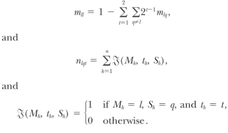
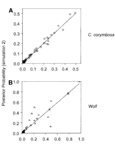
corym-bosa: The plant speciesCentaurea corymbosais currently shown in Figure 2, A and B. If the two chains have converged, the relationship between their posterior found in only six populations in southern France. In a
study byFreville et al. (2001), 228 individuals (mini- probabilities should be linear. The high degree of scat-ter in the plot of 2500 iscat-terations illustrates that the mum population sample size of 20) from these six
popu-lations were genotyped at six microsatellite loci. This chains have not yet converged (Figure 2A). With 3⫻106 iterations, the relationship is much more linear (Figure data set provides a useful test for our method, as the
genetic differentiation between most populations is 2B). A similar plot of the posterior densities of the inbreeding coefficients in two runs of 3⫻106iterations large, likely as a result of limited seed and pollen
dis-persal (Freville et al. 2001). While the geographical also indicates a strong correlation between posterior probabilities estimated from the two independent runs distances between the populations vary, all occur within
a 3-km2 area. Observed pairwise F
Figure2.—Posterior probability densities of the allele frequencies generated from two sep-arate runs of the program. The runs differed in initial random seed and initial values ofm and F. (A and C) The relationship between these runs over the first 2500 iterations, before equilibrium has been reached. (B and D) The relationship between these runs after equilib-rium has been reached. The latter runs consist of 3⫻ 106iterations, a burn-in of 106, and a sampling period of 2000. Allele frequencies are grouped in 0.05 intervals.
The mean posterior probabilities of the immigration low (Figure 4A) or a high migration rate (Figure 4B). Population sample sizes are nearly identical (38 and 40 rates among populations for the C. corymbosadata are
shown in Table 1. Most populations have low migrant individuals, respectively). Both the migration rate and the sample size affect the variance of the posterior prob-proportions (when averaged over the posterior
proba-bilities) with the exception of population E1, which ability distribution; higher migration rates and smaller sample sizes both increase the variance. In Figure 4A, appears to have a large expected proportion of migrants
(m⫽0.25) from population E2. There appears to be a the estimated 95% credible set of values for the allele frequency is (0.50, 0.80) while in Figure 4B it is (0.55, source-sink relationship between the two populations
because the expected proportion of migrants into popu- 0.95). Migration can also cause the mode of the poste-rior density of allele frequency to differ from the maxi-lation E2 from E1 is much smaller (m⫽ 0.00). Figure
4, A and B, presents the posterior densities of the fre- mum-likelihood estimate of allele frequency that would be obtained by using the population sample directly quencies of two alleles in a population with either a
and ignoring immigration as is done in many population assignment tests (e.g.,Paetkauet al. 1995).
Another property of the populations that can be stud-ied is the posterior probability distribution of the total numbers of nonimmigrants, first-generation immigrants, and second-generation immigrants. Figure 5, A–C, shows
TABLE 1
Migration rates amongC. corymbosapopulations
E1 E 2 A Pe Po C r
E1 0.73 0.25 0.00 0.00 0.01 0.00
E2 0.00 0.99 0.00 0.00 0.00 0.00
A 0.00 0.00 0.99 0.00 0.00 0.00
Pe 0.00 0.00 0.00 0.99 0.00 0.00
Po 0.00 0.00 0.00 0.00 0.99 0.00
Cr 0.00 0.00 0.00 0.00 0.00 0.96
Means of the posterior distributions ofm, the migration rate into each population, are shown. The populations into which individuals are migrating are listed in the rows, while the origins of the migrants are listed in the columns. Values along the diagonal are the proportions of individuals derived from the source populations each generation. Migration rates
Figure3.—Posterior probability densities of inbreeding
co-efficients generated from two different runs of the program. ⱖ0.10 are in italics. Standard deviations for all distributions were⬍0.05.
Figure 4.—Posterior probability density of a particular allele over all sampled iterations. (A) Allele 174 from locus 13D10 in population Pe. (B) Allele 163 at locus 13B7 in population E1. (C) The frequency distribution of allele 128, locus cxx140, Fort St. John population. (D) The distribution of allele 200, locus cxx204, Great Bear Lake population. The gray line represents the maximum-likelihood esti-mate for this allele when calculated from indi-viduals sampled from this population. Settings for the MCMC chain are as in Figure 2.
these posterior distributions forC. corymbosapopulation should bemand the proportion of second-generation migrants should be 2m. As no higher orders of migrants E1. The expected proportions of nonimmigrants and
first-generation immigrants overlap, although the vari- are currently considered in our method, the average proportion of nonmigrants should be ⵑ1 ⫺ m ⫺ 2m
ance of the posterior distribution of the proportion of
first-generation migrants is lower. The expected propor- under our model, or in this case, 0.25, which falls near the center of our 95% credible set.
tion of second-generation immigrants is about twice as
high and the variance is also larger (this is likely due Our method can also be used to study the migrant ancestry assignments of individuals, taking account of in part to the fact that assignments of second-generation
immigrants are less certain than those of first genera- overall population migration rates and uncertain popu-lation allele frequencies. Figure 6A shows the posterior tion). The 95% credible set for the proportion of
first-generation migrants is (0.10, 0.45)vs. (0.30, 0.75) for probabilities of nonimmigrant, first-, or second-genera-tion immigrant ancestry for five individuals from popu-second-generation migrants and (0.00, 0.55) for
nonmi-grants. The reason that the probability of the proportion lation E1 and one individual from population E2. In-dividual 4-E1 is most likely to be a first-generation of nonimmigrants being above 0.55 is negligible, while
the migration rate into this population isⵑ0.25 (Table immigrant, individuals 11-E1 and 37-E1 are most likely to be second-generation immigrants, and individuals 1), is outlined inappendix a. The prior predicts that
the expected proportion of first-generation migrants 22-E1 and 31-E1 are roughly equally likely to be either
Figure 6.—Posterior distribution for the as-signment of individuals to ancestry states 0 (䊏), 1 ( ), and 2 (䊐) forC. corymbosaand wolf. All individuals are from the populations examined in Figure 5, except the lastC. corymbosaindividual, which is from E2.
nonimmigrants or second-generation immigrants. Our close to one another, with no obvious physical barriers to gene flow between them (for example, the Tuktoyak-method is able to identify second-generation
immi-grants with a high level of certainty due to the linkage tuk/Inuvik and Paulatuk populations, FST ⫽ 0.009), while others are separated by mountain ranges (Kluane disequilibrium observed in the multilocus genotypes of
individuals whose parents have originated in different National Park), the Arctic Ocean (Banks Island), or large geographic distances (Fort St. John). As such, populations. Individual 1-E2 is most likely to be a
nonim-migrant. Excluding population E1, in only 3 of 190 cases these samples allow us to determine the effect of differ-ences in genetic differentiation on our method’s ability did an individual assign with probability ⬎0.05 to a
population other than the one it was sampled from, to obtain reliable estimates of migration rates and indi-vidual immigrant ancestries.
indicating very low levels of migration.
The posterior probability density of the population To estimate the posterior probability distributions of the parameters the MCMC was run for a total of 3 ⫻ inbreeding coefficient,F, was concentrated near 0 for
most populations, although the standard deviation was 106iterations, discarding the first 106iterations as burn-in. Samples were collected every 2000 iterations to infer large in population E1, which had the greatest amount
of immigration; in that case, the estimated mean of posterior probability distributions of parameters. Figure 1B shows the log-posterior probability plotted against the posterior density was F ⫽ 0.027 but the standard
deviation was 0.39. This is likely a result of the lack of iteration number for the gray wolf data. The increase in log-probability appears to plateau afterⵑ10,000 itera-information available to the method for estimatingF, as
most individuals in this population have high posterior tions. Figure 2, C and D, shows the correlations (be-tween two independent MCMC runs) of the posterior probabilities of being first- or second-generation
mi-grants. The remaining populations had much lower probability densities of each allele frequency, at each locus, in each population (grouped in intervals of 0.05). standard deviations (⬍0.08). The population Pe had
significant posterior probability associated with rela- The high degree of scatter in the plot of 2500 iterations
vs.the plot of 3⫻106iterations (which is highly linear) tively large positive values ofF(mean of posterior density
was F⫽ 0.123 with a standard deviation of 0.05), sug- once again illustrates that the chains have not yet con-verged at 2500 iterations but have the appearance of gesting potential local inbreeding effects.
Application to gray wolf data:In a study of population convergence after 3⫻106iterations. A similar plot (Fig-ure 3B) of the posterior densities of the inbreeding genetic structure of gray wolves,Canis lupus, in the
Cana-dian Northwest, Carmichael et al. (2001) genotyped coefficients in two runs, each with 3 ⫻ 106 iterations, also indicates a strong correlation between posterior nine microsatellite loci in 491 individuals (minimum
sample size of 9 individuals) from nine separate regions. probabilities (suggesting the chains have converged). The means (averaged over posterior probabilities) of This data set is a valuable test of our method, as the
appear quite isolated (Banks Island, Fort St. John, Klu-ane National Park, and Northern Richardson Moun-tains). The remaining five populations all have at least one major source of immigrants. There were some nota-bly large mean migration rates between wolf popu-lations. The mean migration rate from the Northern Richardson Mountains to the Southern Richardson Mountains was 0.22; from Tuk/Inuvik to Great Bear Lake, 0.14; from Tuk/Inuvik to Paulatuk, 0.21; and from the Southern Richardson Mountains to Tuk/Inu-vik, 0.23. All of these populations are relatively close to one another, occurring on the mainland of the north-ern Yukon or the Northwest Territories. However, it is worth noting that most of these populations do not have symmetrical migration rates, suggesting that movement of animals between these regions is predominantly uni-directional. For example, while the mean migration rate from the Northern to the Southern Richardson Moun-tains populations was 0.22, the mean migration rate in the opposite direction was only 0.04. The mean migra-tion rate from Banks Island to Victoria Island was also fairly large at 0.19 while the reverse rate was near zero (see Table 2). These islands are quite close to one an-other and are joined by ice during the winter months. Figure 4, C and D, presents the posterior densities of the frequencies of two alleles in populations with either a low immigration rate and a larger sample size or a high immigration rate and a smaller sample size. In these examples, the sample sizes are quite different be-tween the populations (e.g., 41 individuals for Fort St. John and 22 individuals for Great Bear Lake). Immigra-tion causes the mode of the distribuImmigra-tion to exceed the maximum-likelihood estimate by a considerable amount (Figure 4D) and the variance of the estimated posterior density of allele frequency is also much larger in the example with a smaller sample size and higher migra-tion rate. In Figure 4C the estimated 95% credible set for the allele frequency is (0.35, 0.60) while in Figure 4D it is (0.10, 0.70).
Figure 5, D–F, shows the posterior probability distri-butions of the total proportions of nonimmigrants and first- and second-generation immigrants (from any pop-ulation) for the Southern Richardson Mountains gray wolf population. The mode of the posterior proportion of nonmigrants is much lower than that for the posterior distribution of the proportion of either first- or second-generation migrants. Also, the mode of the posterior distribution of second-generation migrants is roughly twice that of first-generation migrants. The variance of the posterior distributions of first- and second-genera-tion migrant proporsecond-genera-tions is much greater than that of the nonmigrant proportion. The 95% credible sets for the former are (0.20, 0.50) and (0.40, 0.70), respectively,
vs.(0.00, 0.20) for the latter.
Figure 6B shows the posterior probabilities of nonim-migrant, first-, or second-generation immigrant ancestry
TABLE 2 Migration rates among gray wolf populations Northern Banks F ort St. Great Kluane Southern Victoria Richardsons Island John B ear Lake National P ark Richardsons P aulatuk Tuk/Inuvik Island Northern Richardsons 0.93 0.00 0.01 0.00 0.00 0.04 0.00 0.00 0.00 Banks Island 0.00 0.99 0.00 0.00 0.00 0.00 0.00 0.00 0.00 Fort St. John 0.00 0.00 0.99 0.00 0.00 0.00 0.00 0.00 0.00 Great Bear Lake 0.03 0.01 0.02 0.68 0.01 0.09 0.01 0.14 0.00 Kluane National P ark 0.01 0.00 0.03 0.00 0.90 0.04 0.01 0.01 0.00 Southern R ichardsons 0.22 0.01 0.02 0.01 0.01 0.71 0.01 0.02 0.01 Paulatuk 0.00 0.00 0.00 0.00 0.00 0.01 0.68 0.21 0.00 Tuk/Inuvik 0.03 0.01 0.01 0.00 0.00 0.23 0.00 0.72 0.00 Victoria Island 0.01 0.19 0.02 0.02 0.02 0.02 0.02 0.02 0.70 Means o f the posterior d istributions of m , the migration rate into each population, are shown. The populations from which each individual was sampled are listed in the rows, while the populations from which they migrated are listed in the columns. V alues along the diagonal are the p roportions of individuals derived from the source populations each generation. Migration rates ⱖ 0.10 are in italics. Standard deviations for all distributions were ⬍ 0.05.
Mountains population. Individual MP9205 is most likely cies in terms ofFSTby using the standard result for the expected FST at stationarity under the Wright model, to be a nonimmigrant. Individual MP9224 is most likely
to be a first-generation immigrant, individual MP9219 FST⫽1/(4Nm⫹1), and solving for 4Nmin terms ofFST to obtain 4Nm⫽1/FST⫺1. The right-hand side of this a second-generation immigrant, and individual MP9220
is fairly evenly split between being a first- and second- equation was substituted for 4Nm in Equation 4. The simulation results are therefore presented in terms of generation immigrant. The posterior probability density
of the population inbreeding coefficient,F, was concen- FST,m,q, andn. To evaluate the statistical performance of the estimator of migration rates under the simula-trated near 0 for most populations, with the exception
of two populations, Great Bear Lake and Northern Rich- tions we focused on two statistics, the mean square error (MSE) and the bias (seeCasellaand Berger 1990). ardson Mountains, which had significant posterior
prob-ability associated with negative values of F. F was also MSE is a function of both the bias and the variance of the estimator (MSE⫽bias2⫹variance). A decrease in approximately uniformly distributed between ⫺1 and
⫹1 in the Victoria Island population, likely because MSE therefore indicates an improvement in the estima-tor. To evaluate the statistical accuracy of migrant ances-most of the individuals in this population were assigned
as migrants. try assignments we examined the proportion of migrants
from each ancestral class (e.g., nonmigrants, first-gener-ation migrants, and second-generfirst-gener-ation migrants) that
SIMULATION STUDY were assigned to a given class with maximum posterior probability.
Simulation methods:To evaluate the statistical
prop-To examine the performance of the model under erties of the new method we simulated samples from
various conditions, different values were assigned to a populations exchanging migrants according to the
number of parameters. The most common allele in a
Wright(1931) island model (at stationarity). The allele
population (q) was assigned a value of either 0.5 or 0.9. frequencies (assuming biallelic loci) in pairs of
The number of individuals sampled from each popula-tions receiving migrants from a common source, with
tion (n) was either 20 or 100. Populations were sepa-allele frequency qi at locusi, were simulated from the
rated byFSTvalues of 0.01, 0.10, or 0.25. Migration rates stationary probability density function (pdf) under the
between populations (m) were 0.01, 0.05, 0.10, or 0.20. Wright island model. The simulated markers could be
Three different numbers of loci were simulated: 5, 10, SNPs, for example, which are typically biallelic. The pdf
and 20. The parameters listed above were used for simu-of the allele frequency at locusiin populationjis
lations in all possible combinations, for a total of 144 parameter combinations. Each of these combinations
f(pij)⫽
⌫(4Nm)
⌫(4Nmqi)⌫(4Nm[1⫺qi])
pij4Nmqi⫺1(1⫺pij)4Nm(1⫺qi)⫺1.
was replicated 10 times. As each simulated data set con-tained two populations, data were generated for 20 sim-(4)
The pdf of the allele frequencies atJ unlinked loci in ulated populations for each combination of parameter settings. The MCMC was run with the same settings populationiisf(pj)⫽ ⌸if(pij), where the product is over
theJ loci andpj⫽{pij} is the vector of allele frequencies (number of iterations, etc.) as in each of the examples. As the results with q⫽ 0.5 were very similar to those in population j. The alleles at each locus were
there-fore simulated as independent and identically distrib- obtained with q⫽ 0.9, only the former are examined here.
uted with common pdf given by Equation 4. A sample
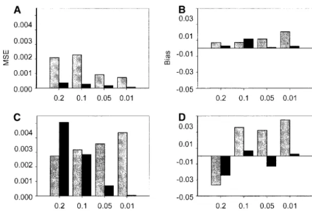
ofnindividuals was generated from each simulated pop- Simulation results:The results of the simulation study are summarized in Figures 7–10. Figure 7 shows the ulation according to the multinomial sampling
distribu-tion of Equadistribu-tion 2. It was assumed that (recent) migra- influence of the number of loci and the migration rate used for the simulations on MSE and bias of the esti-tion occurs between the two populaesti-tions with ratesm12
and m21. To reduce the number of parameters to be mated migration rate for a fixed degree of genetic differ-entiation (FST ⫽ 0.25). In the case of 5 loci (Figure considered in our simulations, we assumed that m ⫽
m12⫽ m21andqij⫽qfor alli,j. 7D), the data have little influence on the estimates, by comparison with the influence of the prior. The prior If an individual is a nonmigrant, the genotype is
gen-erated by assigning alleles according to the Hardy-Wein- specifies thatmis uniform on the interval (0, 0.33) with mean 0.167. When the actual value of m exceeds the berg proportions, conditional on the simulated allele
frequencies in the population from which the individual mean of the prior (e.g., when m⫽ 0.2), the estimator has a negative bias. When the actual value ofmis less was sampled. A first-generation migrant similarly has its
genotype assigned according to Hardy-Weinberg pro- than the mean of the prior (e.g.,mⱕ0.1) the estimator has a positive bias, as expected if the posterior is essen-portions, but conditional on the allele frequencies in
the alternative population. A second-generation migrant tially similar to the prior. With 20 loci, the data have a greater influence than the prior and we see a smaller has its genotype assigned by drawing an allele from each
frequen-Figure7.—MSE and bias for the migration rate estimate from simulated data. The following pa-rameters were used for data simulation: 5 (C and D) or 20 (A and B) loci, 20 ( ) or 100 (䊏) individuals per population, and migration rates of 0.2, 0.1, 0.05, or 0.01, whenFST⫽0.25.
ber of loci sampled (Figure 7, A and C) and with increas- gree of genetic differentiation between populations (FST ⫽ 0.25) and 20 loci, the mean of the maximum ing sample size, although sample size appears less
impor-tant in this case. posterior probability assignment (across sampled
indi-viduals) increases with decreasing migration rate and It is apparent from our simulation analyses that the
effects of sampling either more individuals or more loci the variance of the maximum posterior probability (across individuals) decreases (Figure 9, A and B). In the are correlated. With a small number of loci, increasing
the sample size (from 20 to 100) has little effect on the case of low genetic differentiation between populations (FST ⫽ 0.01) and 5 loci the migration rate has little bias or MSE of the estimated migration rate (Figure 8,
A and B), but with a larger number of loci (20 loci), influence on the mean or variance of the maximum posterior probability assignments (Figure 9, C and D). increased sample size dramatically reduces bias and
MSE (Figure 8, C and D). Figure 10 examines the accuracy of the individual
migrant ancestry assignments as a function of migration The migration rate and the level of genetic
differenti-ation between populdifferenti-ations also influence the mean rate, sample size, and number of loci when populations with a high degree of genetic divergence (FST⫽ 0.25) (and variance) of the maximum posterior probabilities
(i.e., the highest posterior probability assignment) of are considered. For each of the categories 0 (nonmi-grant), 1 (first-generation mi(nonmi-grant), or 2 (second-gener-individual migrant ancestries. In the case of a high
Figure 9.—Mean and variance of the maxi-mum posterior probability for each individual mi-grant ancestry from simulated data. The following parameters were used for data simulation:FST⫽ 0.25 and 20 loci (A and B) orFST⫽ 0.01 and 5 loci (C and D). Simulations were performed with either 20 ( ) or 100 (䊏) individuals per popula-tion and migrapopula-tion rates of 0.2, 0.1, 0.05, or 0.01.
ation migrant), the total population of individuals actu- and migrant ancestry assignments. Migrant ancestries are most accurate when either a large number of loci ally belonging to that category is represented by the
height of the histogram bar. Each histogram bar is then and individuals are sampled or migration rates are low. divided into three different shades, representing the
proportion of individuals actually belonging to that
cate-DISCUSSION
gory that are assigned to each of the three categories. If
the assignments were perfectly accurate, each histogram In this article, a new Bayesian method is presented bar would be filled with a single shade (corresponding for use with allozyme, microsatellite, RFLP, or SNP to the migrant ancestry class represented by that histo- multilocus genotype data, which allows one to
simulta-gram bar). neously infer recent migration rates, population allele
Of the four cases shown in Figure 10, the cases with frequencies, population inbreeding coefficients, indi-either high migration rate (m⫽0.2) and large samples vidual migrant ancestries, and other parameters of po-of individuals (100) and loci (20) or low migration rate tential interest. Our method should be of interest to and small samples of individuals (20) and loci (5) pro- ecologists assessing the relative importance of specific vide the most accurate assignments (Figure 10, A and patterns of population dynamics in nature, the preva-D). Decreasing the number of loci sampled from 20 lence of male- (or female-) biased dispersal, the impor-to 5 has a large effect in decreasing the accuracy of tance of geographic barriers to dispersal, and so on. assignments (Figure 10, A and B), but increasing the We have applied our method to two previously pub-number of individuals sampled has only a modest effect lished microsatellite data sets for plants (C. corymbosa) on accuracy (Figure 10, B and C). Finally, decreasing and mammals (gray wolves) to illustrate its use. We have the migration rate also has a large effect, improving the shown that for each of these data sets reasonably precise accuracy of the method even when only 5 loci and 20 information about recent migration patterns can be individuals are sampled (Figure 10, C and D). At least extracted. In the case of theC. corymbosadata, a highly part of the explanation for this trend is the fact that asymmetrical pattern of immigration in one pair of pop-with lower migration rates population allele frequencies ulations (E1 and E2) supports the existence of a source-are more accurately estimated (due to the larger propor- sink population structure.
tion of nonmigrants in the sample). Another pattern observed in both example analyses
Figure10.—The proportion of individuals with a migrant ancestry of 0 (䊏), 1 ( ), and 2 (䊐) (size of the vertical bar) who have their maximum posterior probability in each state (proportion of the bar shaded). Data were simulated from a population FST of 0.25. Simulations were per-formed with a migration rate of 0.2 (A–C) or 0.05 (D), 100 (A and B), or 20 (C and D) individuals, and 20 (A) or 5 (B–D) loci.
hood estimates (observed proportions of alleles) in pop- the probabilities of IBD of alleles sampled from different populations (in the case of individuals with mixed mi-ulations experiencing high rates of immigration; it is
therefore important to simultaneously estimate individ- grant ancestry). This could improve performance be-cause the allele frequencies in populations with low ual migrant ancestries and population allele frequencies
as we have done in this article. Failing to do so may levels of differentiation are not independent and geno-type sample information can therefore be effectively increase the likelihood that an immigrant individual is
incorrectly assigned as a nonimmigrant due to incorrect “combined” across populations (through the use of
F-statistics) to provide improved estimates of allele fre-estimation of the allele frequencies within populations.
This study therefore suggests that it may be preferable to quencies (in the extreme case, imagine two populations with no differentiation; a sample from the first popula-estimate migration rates, migrant ancestries, and allele
frequencies simultaneously in population assignment tion can be used to estimate allele frequencies in the second).
tests.
The results of our limited simulation study indicate Another extension of our approach could be to allow immigration rates to vary over time. Posterior probabili-that very accurate estimates of migration rates and
indi-vidual migrant ancestries can be obtained when levels ties under models with constant or variable immigration rates could then be compared, using predictive poste-of genetic differentiation among populations are large,
migration rates are low, and 20 or more loci are exam- rior probabilities (see Bernardo andSmith2000) to test the hypothesis of constant immigration rates during ined. If 5 or fewer loci are examined little information
may be available, even if a large number of individuals the last few generations. This might potentially allow one to directly address the relationship between immi-are sampled. To explore the robustness of migration
rate estimates and assignments for particular data sets, gration and gene flow. Strictly speaking, gene flow in-volves both immigration and local reproduction. If the it may be advisable to carry out preliminary simulations
to determine the expected accuracy of the method, given rates of migration in the current and previous genera-tions are similar this suggests that there is no difference the observed level of genetic differentiation among
pop-ulations. In our simulation study, we considered only in breeding success between residents and migrants (gene flow equals immigration rate), etc.
diallelic loci and it is likely that accuracy may increase
with increasing numbers of alleles (e.g., with microsatel- A disadvantage of our method, as currently formu-lated, is that it allows only the proportions of immigrants lite locivs.SNPs).
There are a number of ways in which the approach in a population to be estimated; it does not allow one to estimate directly the total proportion of individuals presented here could be extended in the future. First,
we have ignored preexisting patterns of genetic differen- that emigrate from a population or the proportion that emigrate from one particular population to another. tiation among populations; our population-specific
in-breeding coefficients consider only identity by descent For example, a small population may have a large pro-portion of the total individuals in the population migrat-(IBD) of alleles (making up genotypes) within
Bernardo, J. M., andA. F. M. Smith, 2000 Bayesian Theory. Wiley, (because of the relative difference in the population
New York.
sizes) and will provide no indication of the large propor- Carmichael, L. E., J. A. Nagy, N. C. LarterandC. Strobeck, 2001 Prey specialization may influence patterns of gene flow in wolves tion of actual emigration from the source population.
of the Canadian Northwest. Mol. Ecol.10:2787–2798. One way to deal with this would be to estimate
emigra-Casella, G., andR. L. Berger, 1990 Statistical Inference. Duxbury tion rates that are corrected for the relative population Press, Belmont, MA.
Cornuet, J. M., S. Piry, G. Luikart, A. EstoupandM. Solignac, sizes (if known). Alternatively, if temporal samples were
1999 New methods employing multilocus genotypes to select collected, with replacement, information from unique
or exclude populations as origins of individuals. Genetics153:
individual genotypes (or mark-recapture tagging) could 1989–2000.
Dawson, K. J., andK. Belkhir, 2001 A Bayesian approach to the be combined with a method such as ours to jointly
identification of panmictic populations and the assignment of estimate population sizes and relative migration rates.
individuals. Genet. Res.78:59–77.
Another assumption of the method is that all popula- Freville, H., F. JustyandI. Olivieri, 2001 Comparative allozyme and microsatellite population structure in a narrow endemic tions exchanging migrants have been sampled. The
ef-plant species,Centaurea corymbosaPourret (Asteraceae). Mol. Ecol. fect of this assumption may be important and a goal of
10:879–889.
future research should be to devise models that allow Gaggiotti, O. E., F. Jones, W. M. Lee, W. Amos, J. Harwoodet al., 2002 Patterns of colonization in a metapopulation of grey seals. some degree of migration from “unobserved”
popula-Nature416:424–427. tions for which no reference allele frequencies are
avail-Gamerman, D., 1997 Markov Chain Monte Carlo: Stochastic Simulation
able. This could likely be done using the flexible MCMC for Bayesian Inference. Chapman & Hall, New York.
Hastings, W. K., 1970 Monte Carlo sampling methods using Markov framework presented here.
chains and their applications. Biometrika57:97–109. To derive the prior probability distribution for
indi-Kingman, J. F. C., 1982 On the genealogy of large populations. J. vidual immigrant ancestries, we have considered the Appl. Prob.19A(Suppl.): 27–43.
Metropolis, N., A. W. Rosenbluth, M. N. Rosenbluth, A. H.
distribution of migrant ancestries in a population in the
TellerandE. Teller, 1953 Equations of state calculations by limit of low migration rates and random mating between
fast computing machine. J. Chem. Phys.21:1087–1091. migrants and residents. Simulation studies are needed Paetkau, D., W. Calvert, I. StirlingandC. Strobeck, 1995
Mi-crosatellite analysis of population structure in Canadian polar to determine the robustness of this approximation in
bears. Mol. Ecol.4:347–354. the face of high migration rates and local inbreeding
Pritchard, J. K., M. StephensandP. Donnelly, 2000 Inference among migrant founders. Despite some outstanding is- of population structure using multilocus genotype data. Genetics
155:945–959. sues of interpretation and reliability, methods for
esti-Rannala, B., andJ. L. Mountain, 1997 Detecting immigration by mating recent migration rates using multilocus
geno-using multilocus genotypes. Proc. Natl. Acad. Sci. USA94:9197– types, such as we have presented here, should provide 9201.
a useful (and complementary) alternative to existing Slatkin, M., andN. H. Barton, 1989 A comparison of three indirect methods for estimating average levels of gene flow. Evolution43:
methods, on the basis of diffusion approximations or
1349–1368.
coalescent theory, aimed at estimating historical migra- Tavare, S., 1984 Line of descent and genealogical processes, and tion rates under particular demographic scenarios. On their applications in population genetics models. Theor. Popul.
Biol.26:119–164. balance, we are optimistic that new methods for
infer-Vitalis, R., andD. Couvet, 2001 Estimation of effective population ring contemporary migration rates and gene flow will size and migration rate from one- and two-locus identity measures. ultimately require fewer assumptions and will yield in- Genetics157:911–925.
Wright, S., 1931 Evolution in Mendelian populations. Genetics16:
formation that is highly relevant to conservation
biolo-97–159.
gists, ecologists, human geneticists, and others dealing Wright, S., 1969 Evolution and Genetics of Populations: The Theory of with practical problems involving recent (or ongoing) Gene Frequencies, Vol. 2. University of Chicago Press, Chicago. migration and admixture among study populations.
Communicating editor: J.Hey
The program BayesAss, written in C, is available from our website at http://rannala.org.
We thank Helene Freville and Isabelle Olivieri for providing us APPENDIX A with their plant microsatellite data and Lindsey Carmichael and Curtis
Expected migrant proportions:Define the probability Strobeck for providing us with their wolf microsatellite data. We are
grateful to the two anonymous reviewers. This research was supported (per generation) that an individual is a migrant as m by the National Institutes of Health grant HG01988 and Canadian and letφbe the expected fraction of alleles at a locus that Institutes of Health research grant MOP 44064 to B.R.
is derived from migrants. By enumerating all possible patterns of ancestry (individual is a migrant, individual is a nonmigrant but both parents are migrants, etc.)
LITERATURE CITED
that result in a given value ofφ, we obtain
Anderson, E. C., and E. A. Thompson, 2002 A model-based
ap-proach for identifying species hybrids using multilocus genetic Pr(φ⫽1)⫽ m⫹ (1⫺m)m2 ⫹. . . data. Genetics160:1217–1229.
Beerli, P., andJ. Felsenstein, 1999 Maximum likelihood
estima-⫽ m⫹ O(m2) . tion of migration rates and effective population numbers in two
populations using a coalescent approach. Genetics152:763–773.
Beerli, P., andJ. Felsenstein, 2001 Maximum likelihood estima- Pr
冢
φ⫽ 12
冣
⫽ 2m(1 ⫺m) 2⫹冢
42
冣
m2(1⫺m)5 ⫹. . . tion of a migration matrix and effective population sizes in n
subpopulations by using a coalescent approach. Proc. Natl. Acad.
Pr
冢
φ⫽14
冣
⫽4m(1 ⫺m) 6 ⫹冢
82
冣
m2(1⫺m)13⫹. . .
⫽ 4m⫹ O(m2) ,
where the notationO(m2) denotes terms of orderm2and higher. The first term in each series is the probability of a single migrant ancestor: In the case of φ ⫽ 1 the individual is a migrant (at generation 1); in the case of φ⫽1⁄
2the individual has a migrant parent (at generation 2); and in the case ofφ⫽1⁄
4the individual has a migrant grandparent (at generation 3). Several possible ances-tries leading toφ⫽1 andφ⫽1⁄
2are shown in Figure A1. The other terms allow possibilities such as two immigrant parents at generation 2 (in the case ofφ⫽1), etc.
The first term in each of the three possibilities listed above (migrant, migrant parent, and migrant grandpar-ent) is a linear function ofm, and the remaining terms are of order m2 and higher. If m is small the higher-order terms can be neglected and we need consider only possibilities involving a single migrant ancestor at some generation (this approximation is implicit in the
FigureA1.—Several possible patterns of immigrant
ances-method ofRannalaandMountain1997). In the limit
try that would each result in either all of an individual’s genes
of smallm, we expect a fractionmof individuals in the
arising from an immigrant source (top of figure,φ ⫽1) or
population to be first-generation migrants, a fraction one-half of an individual’s genes arising from an immigrant 2mto have one migrant parent, a fraction 4mto have source (bottom of figure,φ⫽1⁄
2). Immigrants are denoted by solid circles and nonimmigrants by open circles. The
probabil-one migrant grandparent, and so on. Individuals with
ity of each pattern, given a migration ratemand assuming
migrant ancestry beyond parents will have only
one-random mating, is given below each part.
quarter of their genome derived from migrant ances-tors, on average, and for smaller numbers of loci such individuals will be statistically indistinguishable from
2 p⫽
1
2
关
(p⫺ p0)2⫹(p⫺p m)2
兴
, nonmigrants; we have therefore chosen to use only theprevious two generations of migrant ancestry to estimate
m, although more distant generations could also be
⫽ 1
2
冤冢
p0⫹pm
2 ⫺p0
冣
2⫹
冢
p0⫹pm 2 ⫺ pm冣
2
冥
, included with sufficient numbers of loci.Constant allele frequencies: Assume that a
Fisher-Wright population of constant sizeNereceives migrants ⫽ 1
4⌬p 2 0. at ratem. The deterministic change in allele frequency
in the population due to migration in each generation For a given value ofF
ST, the difference ⌬ptakes on its
is most extreme values whenp ⫽ 1⁄
2and the value of FST is then⌬p2
0. In that case, we can rewrite⌬pas
⌬p⫽⫺m⌬p0,
|⌬p|⫽ m
√
FST. where ⌬p ⫽ p1 ⫺ p0 is the change in the populationWe now have an expression for the magnitude of the allele frequency in a single generation and⌬p0⫽p0⫺
change of allele frequency (per generation) under
mi-pm is the difference in allele frequency between the
gration pressure in a population that receives migrants population that is the migrant source and the
popula-from another population with a specified level of differ-tion from which individuals are sampled. For a single
entiation between the populations. Ifm⬍0.05 andFST⬍ diallelic locus, the measure of population
differentia-0.05 then⌬p⬍0.01 and the change of allele frequency tion,FST, is defined as
over a few generations will be negligibly small. Similarly, twice the standard deviation of the allele frequency
FST⫽
2 p
p(1⫺p) change due to drift will be
(seeWright 1969), where p is the average allele
fre-2p⫽2
冪
p0(1⫺p0)
2Ne
⫽
冪
2p0(1⫺ p0)Ne
. quency across populations and2
pis the variance of allele frequencies across populations. We can write2
pfor our
great-If element mll is chosen, the proposed value is mll* ⫽ est whenp0⫽1⁄2and in that case 2p⫽
√
1/2Ne. IfNe⬎mll[a]⫹z, wherezis chosen on a uniform interval (⫺␦m, 5000 then 2p⬍0.01 and the change of allele frequency
⫹␦m) with reflecting boundaries, where␦mⱕ1⁄3. Ifmll*⬎ over a few generations will be negligibly small. These
1 ormll*⬍2⁄3thenmlq* is reflected back onto the interval values define boundaries beyond which the
approxima-(2⁄
3, 1) by an amountmlq[a]⫹z⫺1 or2⁄3⫺z⫺mlq[a]. tions underlying the proposed method will be well
satis-The remaining elements are adjusted to sum to 1 using fied. In such cases, the resulting estimates should be
the transformation accurate. The method may provide reasonable estimates
for larger values ofmandFST(or smallerNe) as well but
mlj*⫽
mlj(1 ⫺mll*)
兺
j⬆qmlj . the specific range of applicability remains to be shown.Simulation studies are needed to evaluate the
perfor-mance of the method under a range of conditions. We assumed a uniform Dirichlet prior for m and a uniform prior (on the integers 0, 1, 2) fortiso that the terms in the MH ratio involving the priors formandt
APPENDIX B cancel. The nominating functiong(m*|m[a]) described
above is symmetrical so that these terms also cancel MCMC algorithm:The Metropolis-Hastings (MH)
al-from the MH ratio. gorithm (Metropoliset al. 1953;Hastings1970) was
Modifying individual migrant ancestries:The matrix used to numerically calculate the posterior probability
of individual migrant ancestries at iterationa, denoted density of the parameters in our analyses. The basic
by the composite parametersM[a] andt[a], are modi-idea is to construct a Markov chain with a stationary
fied to be M[a ⫹ 1] ⫽ M* and t[a ⫹ 1] ⫽ t* with distribution that is the joint posterior distribution of
probability the parameters to be estimated. This chain is simulated
and samples from the chain are used to make inferences ␣
M,t(M*,t*|M[a],t[a]) about joint or marginal posterior probabilities of
param-eters. The implementation of the MH algorithm used ⫽
min
冦
1, Pr(M*,t*|m)Pr (X|S;M*,t*,F,p)g(M[a],t[a]|M*,t*) Pr(M[a],t[a]|m)Pr (X|S;M[a],t[a],F,p)g(M*,t*|M[a],t[a])冧
,in our program has four steps at each iteration of the chain. At each step (outlined below) a particular set of
parameters are potentially modified. where
Modifying population migration rates:The matrix of
population migration rates at iteration a, denoted as g(M[a],t[a]|M*, t*)
g(M*,t*|M[a],t[a])⫽
nl*q*t*⫹1
nlqt . m[a], is modified to bem[a⫹1]⫽m* with probability
The nominating functiong(M*,t*|M[a],t[a]) is as
fol-␣m(m*|m[a])⫽ min
冦
1,Pr(M,t|m*)
Pr(M,t|m[a])
冧
. lows: Choose one of thensampled individuals to have its migrant ancestry modified with uniform probability The nominating function g(m*|m[a]) is as follows: 1/n. There are 2I ⫺ 1 possible states for the migrant Choose one of theI2elements of the migration matrixancestry of the chosen individual; it can be a nonmigrant to be modified with uniform probability 1/I2. The
mi-or a first- mi-or second-generation migrant from one of gration rates are constrained by our model such that the remainingI⫺1 populations. The proposed change for an individual must be to one of the 2I⫺2 states other
mll⫽1⫺
兺
q⬆l
(mlq⫹2mlq) ⫽1⫺3
兺
q⬆l
mlq and mllⱖ0 .
than its present state and each possibility is assigned a uniform probability 1/(2I⫺2).
Modifying population allele frequencies:The matrix It follows that
of population allele frequencies at iterationa, denoted asp[a], is modified to bep[a⫹1]⫽p* with probability 1⫺3
兺
q⬆l
mlq ⱖ 0,
兺
q⬆l
mlqⱕ
1
3, mll僆
冢
2 3, 1冣
.␣p(p*|p[a])⫽min
冦
1,Pr(X|S;M,t,F,p*) Pr(X|S;M,t,F,p[a])
冧
. To maintain these constraints, we used the followingproposal scheme. If elementl,qis chosen (l⬆q), the
The nominating function g(p*|p[a]) is as follows: proposed value is mlq* ⫽ mlq[a]⫹ z, where zis chosen
Choose one of theIpopulations with uniform probabil-on a uniform interval (⫺␦m,⫹␦m) with reflecting
bound-ity 1/I, choose one of theJloci with uniform probability aries, where ␦m ⫽ max{0.10, 1 ⫺ mll}. If mlq* ⬎ 1⁄3 or
1/J, and choose one of thekljalleles at locusjin
popula-mlq*⬍0 thenmlq* is reflected back onto the interval (0,
tionlwith uniform probability 1/klj. If alleleiat locus 1⁄
3) by an amount mlq[a]⫹z ⫺1⁄3or ⫺z ⫺mlq[a]. The
jin populationlis chosen the proposed value ispijl*⫽ remaining elementsj⬆qof rowlare adjusted so that
pijl[a]⫹z, wherezis chosen on a uniform interval (⫺␦p, they sum to 1 by using the transformation
⫹␦p) with reflecting boundaries and the remaining al-lele frequencies are adjusted so that the proposed alal-lele
mlj* ⫽
mlj(1⫺ mll ⫺mlq*)
兺
j⬆q,j⬆lmlj, for allj⬆q,j⬆ l.
Modifying population inbreeding coefficients: The types for each individual, the proposed genotypes at these loci at iterationa, denoted asX⫺[a], were
modi-vector of population inbreeding coefficients at iteration
fied to beX⫺[a ⫹1]⫽ X⫺* with probability a, denoted as F[a], is modified to be F[a ⫹ 1] ⫽ F*
with probability
␣X⫺(X⫺|X⫺[a])⫽min
冦
1,Pr(X⫹,X⫺*|S;M,t,F,p) Pr(X⫹,X⫺[a]|S;M,t,F,p)
冧
.␣F(F*|F[a])⫽min
冦
1,Pr(X|S;M,t,F*, p) Pr(X|S;M,t,F[a],p)
冧
.The nominating function g(X⫺*|X⫺[a]) is as follows:
The nominating functiong(F*|F[a]) is as follows: Choose Choose any one of theLT ⫽兺Liloci with missing data one of the I populations with uniform probability 1/I. with uniform probability 1/LT, whereLiis the number The proposed value isFl* ⫽Fl[a]⫹z, wherezis chosen of loci with missing data for individual i. Modify the on a uniform interval (⫺␦F,⫹␦F) with reflecting bound- locus to become genotypeu,vwith uniform probabili-aries such thatFl* remains on the interval (⫺1,⫹1). ties 2/[kl(kl ⫺ 1)] ifu ⬆ vand 1/kl2 ifu ⫽ vwhere kl Modifying genotypes with missing data: If X⫺ is a is the number of alleles (in all sampled populations) at