DOI: 10.1534/genetics.106.065599
Mapping Quantitative Trait Loci for Expression Abundance
Zhenyu Jia and Shizhong Xu
1Department of Botany and Plant Sciences, University of California, Riverside, California 92521 Manuscript received September 5, 2006
Accepted for publication February 11, 2007
ABSTRACT
Mendelian loci that control the expression levels of transcripts are called expression quantitative trait loci (eQTL). When mapping eQTL, we often deal with thousands of expression traits simultaneously, which complicates the statistical model and data analysis. Two simple approaches may be taken in eQTL analysis: (1) individual transcript analysis in which a single expression trait is mapped at a time and the entire eQTL mapping involves separate analysis of thousands of traits and (2) individual marker analysis where differentially expressed transcripts are detected on the basis of their association with the segregation pattern of an individual marker and the entire analysis requires scanning markers of the entire genome. Neither approach is optimal because data are not analyzed jointly. We develop a Bayesian clustering method that analyzes all expressed transcripts and markers jointly in a single model. A transcript may be simultaneously associated with multiple markers. Additionally, a marker may simultaneously alter the expression of multiple transcripts. This is a model-based method that combines a Gaussian mixture of expression data with segregation of multiple linked marker loci. Parameter estimation for each variable is obtained via the posterior mean drawn from a Markov chain Monte Carlo sample. The method allows a regular quantitative trait to be included as an expression trait and subject to the same clustering assignment. If an expression trait links to a locus where a quantitative trait also links, the expressed transcript is considered to be associated with the quantitative trait. The method is applied to a microarray experiment with 60 F2mice measured for 25 different obesity-related quantitative traits. In the experi-ment,40,000 transcripts and 145 codominant markers are investigated for their associations. A program written in SAS/IML is available from the authors on request.
T
HE recently developed microarray technology al-lows us to measure the expression of many genes or transcripts in a single chip. The transcript abundance can be treated as a classical quantitative trait and thus mapping can be done on the transcript. Mendelian loci in the genome that control the expression levels of transcripts are called expression quantitative trait loci (eQTL). In eQTL analysis, an expression trait is mapped to genomic locations represented by cis- or trans-loci. Thecis-eQTL represent sequence variants that encode transcriptional differences (Hubner et al. 2005). Thetrans-eQTL, however, represent remote genes that
regulate the expression of the gene being transcribed
(Yvertet al. 2003). The purpose of a linkage study is to
identify the cis- and trans-eQTL for each transcript. Results from the eQTL analysis may provide more detailed information about the biological processes of the gene network than the classical quantitative trait analysis. Regular quantitative traits are often gross clinical measurements and may be far remote from the
biological processes giving rise to the clinical traits (Schadtet al. 2003).
In eQTL analysis, we often deal with thousands of expression traits simultaneously. Methods developed for multiple-quantitative trait QTL mapping may not apply here because of the high dimensionality of the model. Two simple approaches may be taken in eQTL analysis: (1) individual transcript analysis in which a single expression trait is mapped at a time and the entire eQTL mapping involves separate analysis of thousands of traits and (2) individual marker analysis where dif-ferentially expressed transcripts are detected on the basis of their association with the segregation pattern of an individual marker and the entire analysis requires scanning markers of the entire genome. The first ap-proach requires only known single-trait QTL mapping procedures, e.g., interval mapping (Lander and B ot-stein1989), composite-interval mapping (Jansen1993;
Zeng 1994), or multiple-QTL mapping (Kao et al.
1999). A common practice for handling thousands of transcript traits is to select a small number of target transcripts on the basis of some criterion for preselec-tion and map QTL only for these prescreened tran-scripts (Lanet al. 2003). The second approach requires
only a method for differential expression analysis, 1Corresponding author: Department of Botany and Plant Sciences,
University of California, 900 University Ave., Riverside, CA 92521-0124. E-mail: [email protected]
e.g., the regularizedt-test (SAM) (Tusheret al. 2001),
the hierarchical mixture model of Newtonet al. (2004),
or the model-based cluster analysis (Pan 2002). In
differential expression analysis, one requires samples from at least two conditions, the control and the treat-ment. When applied to expression–marker association studies, the conditions become the marker genotypes,
e.g., individuals carrying one genotype are arbitrarily designated as the control and those carrying the other genotypes as the treatments. When applied to an F2 design where three groups (genotypes) are present, differential expressions are presented in two forms. One is for the ‘‘additive’’ effect where control and treat-ment represent the two homozygotes. The other is for the ‘‘dominance’’ effect where control and treat-ment represent the homozygote (both types) and the heterozygote.
It appears that eQTL mapping has been treated as either a QTL mapping problem for multiple traits or a microarray differential expression problem for multi-ple treatment comparisons. Other than the method described in Kendziorskiet al. (2006), no unique
me-thod has been particularly designed for eQTL analysis. Neither the first nor the second aforementioned sim-ple approach is optimal because data are not analyzed jointly. The mixture over marker (MOM) approach devel-oped by Kendziorskiet al. (2006) is the first attempt to
analyze transcripts and markers jointly. The method is called MOM because the expression level of a transcript is described by a mixture model over markers. A tran-script is either associated with a marker or not associated with any markers at all. Given that the transcript is associated with a marker, it is associated with one and only one of the markers. We believe that the assumption of a transcript associated with at most one marker is too stringent and needs to be relaxed. The MOM approach is able to detect either thecis-locus or one of thetrans -loci, but not both. This seriously limits the application of the MOM method.
In this study, we propose a novel statistical method that combines the two simple approaches into a single step of analysis so that parameters are inferred using multiple transcripts and markers simultaneously. This joint approach captures the maximum information from the microarray experiment. Like a regular quanti-tative trait, a transcript can be mapped to many different locations, includingcis- andtrans-loci. In multiple-QTL mapping, we face a variable selection problem. To avoid variable selection, we have adopted the Bayesian shrink-age analysis, in which marker loci of the entire genome are evaluated simultaneously (Wanget al. 2005).
Mark-ers with small effects are forced to shrink their effects to zero and markers with large effects are subject to no shrinkage. The shrinkage estimation is made possible through Bayesian hierarchical modeling (Gelman2005).
In this study, eQTL parameters are estimated under the framework of shrinkage analysis.
THEORY AND METHODS
Hierarchical linear model: LetGbe the number of
transcripts measured from N subjects of a mapping population. Let M be the number of markers whose genotypes are measured for all the subjects. We now define the following variables. For thekth individual, let
yikbe the expression level of transcriptiandxjkbe the
genotype indicator of marker j, for i¼1;. . .;G,
j¼1;. . .;M, andk¼1;. . .;N. The genotype indica-tor variable is defined as xjk¼{1, 1} for a backcross
(BC) individual orxjk¼{1, 0, 1} for an F2individual for k¼1;. . .;N. Note that, for simplicity, only the additive effect is considered for an F2population in the current study. The expression levelyikcan be expressed as
yik¼ai1
XM
j¼1
xjkgij1eik; ð1Þ
whereaiis the intercept for theith transcript,gijis the
effect of thejth marker on theith transcript, andeikis
the residual error with an assumedN(0,s2) distribution. Model 1 can be rewritten in a matrix notation,
Yi¼
XM
j¼1
Xjgij1ei: ð2Þ
In model 2,Yi ¼ ½Yi1;. . .;YiNTis anN31 vector for the
expression levels of transcripti, andXj ¼ ½Xj1;. . .;XjNT
is anN31 vector for the genotype indicator variables of locusj, where bothYiandXjare assumed to have been
centered (deviations of the original measurements from the mean) and thusPNk¼1Yik ¼0 and
PN
k¼1Xjk¼0 for i¼1;. . .;G andk¼1;. . .;N. Because of this, there is no intercept in the current linear model. Leteibe anN3
1 vector of the residual errors, andeiN(0,Rs2). Note
that R is a known positive definite matrix. It is not an identity matrix because covariances among the residual errors have been introduced when the intercept is re-moved Quand Xu(2006). Given all thegijvariables, the
probability density ofYiis pðYij
X
Xjgij;Rs2Þ ¼NormalðYi; X
Xjgij;Rs2Þ; ð3Þ
where we use a notation Normal(x;b,d) orN(x;b,d) to denote a normal density for vectorxwith meanb and variance matrixd. In subsequent sections, we adopt the same notation for other probability densities,i.e.,
pðvariablejparameter listÞ
pðgijjhij;s2jÞ ¼ ð1hijÞNðgij;0;dÞ1hijNðgij;0;s2jÞ; ð4Þ whered¼104(a small positive number) ands2
j is an
unknown variance assigned to the jth locus. Variable
hij¼{0, 1} is used to indicate whethergijis sampled from
aN(0,d) or aN(0,s2
j) distribution. If it comes from the
first normal distribution,gijis virtually fixed at zero. If it
comes from the second normal distribution (the distri-bution with a large variance),gijhas a nontrivial value and should be estimated from the data. Therefore,hij¼ 1 means that locusjis an eQTL for transcripti. In some of the literature (e.g., Zhanget al. 2005), the mixture
distribution is described as
pðgijjhij;s2jÞ ¼ ð1hijÞdðgijÞ1hijNðgij;0;s2jÞ; ð5Þ whered(gij) is the Dirac delta function (originally
intro-duced by the British theoretical physicist Paul Dirac) that has the value of‘ for gij¼ 0 and the value zero
elsewhere. The Dirac delta function is actually a prob-ability density function. Therefore, the integral of the delta function from‘to1‘is 1. The above mixture distribution says thatgijhas a nonzero probability mass at the value zero and a quite flat normal distribution around zero provided thats2
j is large. This distribution
is called the spike and slab distribution (Mitchelland
Beauchamp 1988). When d ¼ 0, the two forms of
mixture distribution are identical. We further describe
hij by a Bernoulli distribution with probability rj,
denoted by Bernoulli(hij;rj). Because of the
hierarchi-cal nature of the model, we can further describerjby a
Dirichlet distribution, denoted by Dirichlet(rj; 1, 1).
The parameter rj will control the proportion of the
transcripts that are associated with markerj. All tran-scripts that are assigned to the second component of the mixture distribution are associated with thejth marker. The variance of the genes in this cluster is assigned a scaled inverse chi-square distribution, denoted by Invx2ðs2
j;d0;v0Þ, whered0¼5 andv0¼50 are used
in this study. The residual variance is assigned a vague prior;i.e., Invx2(s2; 0, 0)¼1/s2. This vague prior may cause an improper posterior (Hobert and Casella
1996). In practice, this vague prior has been used all the time and people rarely see any problems. We used a proper scaled inverse gamma distribution for one case of the simulation to test the difference between the vague prior and the proper prior and did not see any notable difference (data not shown).
Markov chain Monte Carlo:Given the likelihood and
the prior of parameters, we are ready to infer the pos-terior distribution of the parameters. Because the form of the posterior distribution is intractable, we use Markov chain Monte Carlo (MCMC) sampling to draw a posterior sample from which empirical posterior means of interested parameters can be found. The most important parameters in the eQTL mapping arehijand
rj. The posterior mean of hij represents the
prob-ability that transcript iis associated with markerj. The posterior mean of rj reflects the proportion of
tran-scripts that are associated with markerj. In addition to these parameters, other parameters may also be inter-esting. For example, the posterior mean ofgijrepresents
how strongly marker j affects the expression of tran-scripti,i.e., the size of the eQTL.
First, we choose an initial value for each variable. We then derive the distribution of one variable conditional on the data and values of all other variables. This distri-bution is called the conditional posterior distridistri-bution, denoted by p(uk j data, uk), where uk is the current variable of interest and ukis the list of the remaining variables (excludinguk). This distribution usually has a
simple form from which a realized value for ukis
sam-pled. Once each and every variable is updated, we com-plete one iteration or sweep. The sampling process continues until the Markov chain reaches its stationary distribution. Convergence diagnosis was conducted us-ing the R package ‘‘coda’’ (Rafteryand Lewis1992). We
discard a number of iterations from the beginning of the chain (burn in) and save one observation in every 10 sweeps of the remaining iterations to form a posterior sample until the posterior sample is sufficiently large to allow an accurate estimate of the posterior mean for each variable. We now describe the sampling algorithm for each variable:
1. Variablehijis simulated from Bernoulli(hij;pij), where
pij ¼ rjNðgij;0;s 2
jÞ
rjNðgij;0;s2jÞ1ð1rjÞNðgij;0;dÞ: ð6Þ
2. Variablegijis simulated fromN(gij;mg,s2g), where
mg¼ XjTR1Xj1
s2 hijs2j1ð1hijÞd
" #1
XjTR1DYi; ð7Þ
s2g¼ XjTR1Xj1
s2 hijs2j 1ð1hijÞd
" #1
s2; ð8Þ
and
DYi¼Yi
XM
j96¼j
Xj9gij9; ð9Þ
which is called the offset of Yi adjusted for the jth
marker effect. 3. Samples2
j from
Invx2 s2j;X
G
i¼1
hij1d0;X
G
i¼1
hijg2ij1v0
!
4. Samples2from
Invx2 s2;GN;X
G
i¼1 ðYi
XM
j¼1
XjgijÞTR1ðYi
XM
j¼1
XjgijÞ !
:
5. Simulaterjfrom
Dirichlet rj;X
G
i¼1
hij11;GX
G
i¼1
hij11
!
:
So far, every variable has been updated. Let
hij¼N1 p
PNp
l¼1h
ðlÞ
ij be the posterior mean of variable
hij, where Np is the posterior sample size. Transcript
i is said to be associated with marker j if the pos-terior probabilityhij is greater than some prespecified threshold. It has been shown that the false discovery rate (FDR) can be controlled ata100% if the appro-priate threshold is the smallest posterior probabil-ity such that the average posterior probabilprobabil-ity of all transcript–marker linkage exceeding the threshold is
.1 a (Efron 2004; Newton et al. 2004). In the
current study, 0.8 is taken as the cutoff point. The 0.80 criterion is somewhat arbitrary and another value, say 0.90, may be used. In theapplicationsection, we show
that any value between 0.6 and 1 is reasonable. This criterion does not affect the MCMC process other than the list of transcripts declared as being associated to markerj.
Missing markers: The algorithm described above
applies to the situation where the genotypes of markers are known for all individuals. In reality, the genotypes of some markers may be missing for some individuals. This means that some elements ofXjare also variables (data
not observed) and subject to the same MCMC sampling as other variables. In this case, we adopt the usual sam-pling procedure in Bayesian mapping to simulate the missing genotypes (Raoand Xu1998). First, all missing
genotypes are sampled from their Mendelian prior distribution: 50% probability of taking either genotype for a BC individual or {25%, 50%, 25%} probability of taking one of the three genotypes for an F2individual. Given the sampled missing genotypes, all marker geno-types are presumably known. We can now start the MCMC process by updating the missing values one at a time from its conditional posterior distribution given the two flanking marker genotypes and all other in-formation available at the current stage of the MCMC process. The process of marker genotype imputation is the same as that described by Sen and Churchill
(2001) and implemented in R/QTL (Broman et al.
2003). The conditional posterior distribution is briefly described below.
Consider that the genotype of markerjis missing for individualk. Letp(YjX) be the probability density of the expression levels for all transcripts measured from
individualkgiven the genotype at markerj. Of course,
Xcan take up to two different values for a BC individual or three different values for an F2individual. Letp(MLj
X) andp(MRjX) be the probabilities for the left and the right flanking markers, respectively, conditional onX. Note that the order of the three markers isML,X,
MR. Let p(X) be the Mendelian prior probability for
the genotype of the missing marker. The conditional posterior probability is defined as
pðXjY;ML;MRÞ
¼P pðXÞpðMLjXÞpðMRjXÞpðYjXÞ X9pðX9ÞpðMLjX9ÞpðMRjX9ÞpðYjX9Þ
; ð10Þ
where PX9 means summation over all possible values
of X9. This probability is used to simulate a realized value ofX.
Heritability for a transcript: In the eQTL analysis,
each transcript has been treated as a quantitative trait. Since the variance of a quantitative trait can be parti-tioned into a genetic variance component and an envi-ronmental variance component, the variance of an expression trait can be similarly partitioned. We now give the formula for calculating the variance com-ponents for each expression trait as a function of the eQTL effects and then further derive the average variance components for all expression traits in the entire microarray experiment. These variance compo-nents are further used to calculate the ‘‘heritability’’ of a transcript.
Lets2
Yibe the variance of transcriptiover all subjects
(a total ofN subjects). Lets2
Xj be the variance of
vari-able Xj over all subjects for marker j. Let us further
definesXjXj9 as the covariance betweenXjandXj9across subjects, i.e., the covariance between markersj and j9
forj96¼j. The variance of transcriptiis expressed as
s2Y
i ¼
XM
j¼1
g2ijs2X
j12 X
j9 .j
gijgij9sXjXj91s
2: ð11Þ
For a BC design,s2
Xj ¼1 andsXjXj9 ¼12rjj9, whereas for an F2design,s2
Xj ¼
1
2andsXjXj9 ¼ 1
2ð12rjj9Þ, where rjj9is the recombination fraction between markersjand j9. Let
s2G
i ¼
XM
j¼1
g2ijs2X
j12 X
j9 .j
gijgij9sXjXj9 ð12Þ
be the genetic component ofs2
Yi. The heritability for
transcriptiis
h2i ¼ s
2 Gi
s2G
i1s
2: ð13Þ
The average heritability of all transcripts may simply take the averageh2
i across all transcripts. However, there
transcripts. This type of overall heritability is defined as follows. First, we need to partition the expected variance of a transcript into variance components as shown below:
E½s2
Yi ¼
XM
j¼1
E½g2
ijs2Xj12 X
j9 .j
E½gijgij9sXjXj91s2: ð14Þ
The expectation is taken with respect to the eQTL effects. Let s2
Y ¼E½s
2
Yi be the overall variance of the
transcripts. The mixture distribution of gij leads to E½g2
ij ¼rjs2j, where rj is the proportion of transcripts
that are linked to locusj. Because gijandgij9are
inde-pendent, we haveE[gijgij9]¼0. Therefore, the above
equation becomes
s2Y ¼X
M
j¼1
rjs2js2X
j1s
2: ð15Þ
Lets2
G¼
PM
j¼1rjs2js2Xj be the genetic variance
compo-nent. The overall heritability is
h2¼ s
2 G
s2G1s2: ð16Þ
This overall heritability of transcripts is different from the average heritability across all transcripts.
APPLICATIONS
Simulation studies: We carried out two simulation
experiments to compare the performance of the pro-posed method (hereafter designated as BAYES) and the MOM approach (Kendziorskiet al. 2006). In the first
experiments, 10 markers were evenly placed on a 360-cM genome,i.e., 40 cM per interval. Genotypes of markers for each subject were simulated on the basis of the Haldane map function (Haldane 1919). Four eQTL
were placed at markers 1, 3, 6, and 10;i.e., the segregation of these four markers affected the expression of some transcripts. We simulated 50 subjects and 1000 transcripts among which transcripts 605–610 were affected by eQTL at marker 1, transcripts 601–604 were affected by eQTL at marker 3, transcripts 961–1000 were affected by eQTL at marker 6, and transcripts 1–50 were affected by eQTL at marker 10. Note that a transcript was either associated with one eQTL or not associated with any of them. In eQTL analysis, a marker is claimed as an eQTL if it affects at least one transcript and a linkage is defined as a transcript–marker association. For example, in the first simulation experiment, there were a total of four eQTL and 100 linkages. The eQTL effects for the 100 linked transcripts (gij) were simulated from Normal(gij; 0, 32).
The residual error was sampled from Normal(eij; 0, 0.12),
such that the expected heritability for a transcript was 0.90. We chose this small residual variance because MOM
did not work well when the residual variance was large. When the residual variance was large, MOM either declared all transcripts as differentially expressed or did not run by throwing out an error message. The experi-ment was replicated 20 times. We used two methods to analyze the 20 replicated data sets. For the BAYES method, the threshold may be chosen to bound the pos-terior expected FDR ata100% as described intheory and methods. The average threshold value of the 20
replicates was 0.55 when the expected FDR was set to 1%, indicating that any value between 0.6 and 1 can serve as a reasonable threshold value to achieve the controlled FDR. We used 0.8 as the threshold value throughout the entire experiments.
The length of the chain required for convergence was determined by the R package coda. In the current MCMC diagnosis, the quantile to be estimated was set to 0.1, the margin of error of the estimate was 0.05, the probability of obtaining an estimate in the desired interval was 0.95, and the precision for the estimate of time to convergence was 0.001. The diagnosis indicated that 1800 iterations were sufficient to achieve conver-gence. Another issue that sometimes arises is the high posterior correlations or the so-called ‘‘stickiness’’ of the MCMC algorithm. The commonly utilized approach to circumvent this problem is to use every kth simulation draw, for some value of k such as 10, 20, or 50 (see Raftery and Lewis 1992 and Gelman et al. 1995 for
more details). In our study, we deleted 1000 iterations as a ‘‘burn-in’’ period and thereafter kept one observation in every 10 iterations until the posterior sample size reached 200. The overall length of the chain was 3000, much longer than the required length of 1800 reported from the coda diagnosis.
The MOM analysis actually consists of two steps: (1) identifying differentially expressed (DE) transcripts and (2) localizing eQTL for each differentially expressed transcript. In the first step, a transcript is identified as DE if the posterior probability of equivalent expression (EE) is smaller than some threshold, where thresholds are chosen to control the FDR at 5%. In the second step, the 90% highest posterior density (HPD) region was used to specify linkages between each transcript and markers. Both methods successfully detected four eQTL and 98 linkages on the basis of the analysis of 20 repli-cates. The two missed linkages were represented by asso-ciations between transcript 605 and marker 1 and between transcript 26 and marker 10, respectively. The true effects for the two linkages were 0.035 and 0.014, which are too small to be detectable with any reasonable analysis methods. Neither method detected any false linkages. The estimated proportions (rj) of transcripts
The normalized average evidence (NAE) of linkage was defined as the average posterior probability over tran-scripts and normalized by the sum of the evidence over all markers (Kendziorski et al. 2006). The estimated
proportions (rj) in the BAYES method, which are
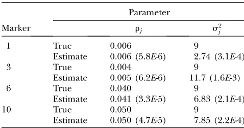
equivalent to the NAE used in the MOM analysis, can be used to sift hot-spot regions where the transcripts are mapped. This simulation demonstrates that both meth-ods are adequate if a transcript is affected by at most one eQTL. The estimated parameters and the effects of the 98 detected linkages used in the simulation experi-ments are provided in Table 1 and also illustrated in Figure 2. The estimated parameters and the effects of eQTL are very close to the true values used to generate
the data. Note that the sample size for the linked tran-scripts was very small (#50) for each eQTL. As a result, the estimated s2
j’s showed some deviations from the
true value of 9.
In the second simulation experiment, we used the same marker map and eQTL setting as in the first exper-iment and generated 20 replicates. In this case, however, we let the eQTL at marker 1 control transcripts 1–20 and transcripts 971–990 and let the eQTL at marker 3 control transcripts 17–20. The transcripts controlled by the eQTL at markers 6 and 10 remained the same as in the first experiment. The purpose of the second simulation experiment was to allow some transcripts to be controlled by more than one marker. For example, transcripts 1–16 were controlled by markers 1 and 10, transcripts 971–990 were controlled by markers 1 and 6, and transcripts 17–20 were controlled by markers 1, 3, and 10. Again, we sampled all the eQTL effects from Normal(gij; 0, 32) and the residual error from Normal (eij; 0, 0.12), such that the expected heritability for a
transcript is 0.92. For the sake of comparison, we used the empirical type I and type II errors and the empirical statistical power to evaluate the performance of our method (BAYES) and the MOM method. The current simulation experiment contains 134 linkages. The BAYES analysis detected 133 linkages and no false positives were declared. Therefore, the empirical type I error was zero, the type II error was 1
134¼0:007, and the empirical power was 1 0.007 ¼0.993. When we examined the single missed linkage (transcript 2 asso-ciated with marker 10), we found that the true marker effect for this transcript was 0.055, which again might be too small to be detected by any reasonable methods. Figure 1.—Hot-spot regions along the chromosome for
the first simulation experiment. NAE, normalized average evidence.
Figure2.—Effects of 98 linked transcripts in the first
sim-ulation experiment. Solid and dashed bars represent the true and the estimated values ofgij, respectively.
TABLE 1
Posterior mean and posterior variance (in parentheses) ofrjanda2j from the Bayes analysis for
the first simulation experiment
Parameter
Marker rj s2j
1 True 0.006 9
Estimate 0.006 (5.8E-6) 2.74 (3.1E-4)
3 True 0.004 9
Estimate 0.005 (6.2E-6) 11.7 (1.6E-3)
6 True 0.040 9
Estimate 0.041 (3.3E-5) 6.83 (2.1E-4)
10 True 0.050 9
Estimate 0.050 (4.7E-5) 7.85 (2.2E-4)
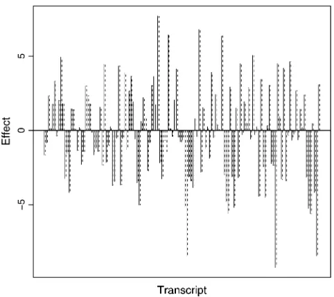
The true parameters used in the simulation and their estimated vales obtained from the proposed method are given in Table 2. The true and the estimated effects for the 133 detected linkages are illustrated in Figure 3. The estimates agree well with the true values. The hot-spot regions represented by the estimated proportions (rj)
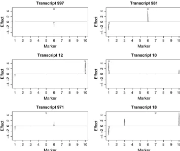
of transcripts associated with the 10 markers are shown in Figure 4 (the top plot). All 4 markers controlling the expression of transcripts have been identified. A strik-ing advantage of the new method over MOM is that an individual linkage picture can be obtained when we focus on a specific transcript. The estimated marker effects for 6 of the detected transcripts are plotted in Figure 5, showing a close agreement to the true values. In the MOM analysis, however, many true linkages have been missed (see Table 3) because each transcript was
allowed to link to at most one locus. The MOM method worked well if a transcript is linked to only one marker,
e.g., transcript 997 associated with marker 6 (see Figure 5). When a transcript is controlled by more than one marker, the linkage signal occurs only at the position where the greatest eQTL resides. For example, tran-script 10 was controlled by markers 1 and 10. The linkage occurred only at marker 1 (true effect 4.462) with marker 10 (true effect 1.510) being completely missed. Transcript 12 was also controlled by markers 1 and 10 whose true effects were 0.997 and 4.489, respectively. MOM detected marker 10 for this tran-script. If the effects of markers controlling the same transcript are similar, MOM generates a confusing result, as demonstrated by transcripts 971 and 18. In the bottom plot of Figure 4, markers 5 and 7 were falsely identified as eQTL by MOM. That marker 6 had a higher peak than marker 1 was also incorrect. The empirical type I error was98664 ¼0:0004 and the power was 1 48
134¼0:642 for the MOM analysis. The power would be even lower if more multiple linkages had been simulated.
The residual variance used in the above two simula-tion experiments was too small, leading to a irrasimula-tionally high expected heritability. In the following simulation experiments, we kept everything the same as that used for the second simulation experiment except residual variance. We varied the residual variance from 0.12to 32, withs2¼0.52, 12, 1.52, 22, 2.52, 32. Again, for each of the six scenarios, we generated 20 replicated data sets. The corresponding expected heritabilities are 0.81, 0.56, 0.32, 0.17, 0.15, and 0.07, respectively. We used only the proposed method (BAYES) to analyze these data sets Figure 4.—Hot-spot regions along the chromosome for
the second simulation experiment. NAE, normalized average evidence.
Figure3.—Effects of 133 linked transcripts in the second
simulation experiment. Solid and dashed bars represent the true and the estimated values ofgij, respectively.
TABLE 2
Posterior mean and posterior variance (in parentheses) ofrjands2j from the BAYES analysis for
the second simulation experiment
Parameter
Marker rj s2j
1 True 0.040 9
Estimate 0.042 (2.9E-5) 5.72 (3.3E-4)
3 True 0.004 9
Estimate 0.005 (6.1E-6) 6.43 (1.1E-3)
6 True 0.040 9
Estimate 0.041 (3.7E-5) 10.9 (2.1E-4)
10 True 0.050 9
Estimate 0.049 (4.5E-5) 13.3 (2.9E-4)
because MOM did not work whens2.0.12. From Figure 6, we can see that the empirical power decreased dramatically as the residual variance increased. The empirical type I error increased accordingly, but not as much as the decrease in the empirical power due to the stringent control for the FDR.
Mice data analysis: We analyzed a mice data set
pub-lished by Lanet al. (2006). The data are publicly
avail-able at gene expression omnibus (GEO) with accession no. GSE3330. The data consist of 40,738 transcripts whose expression levels were measured from 60 F2(ob/ob) mice in an obesity-related research. The expression levels were normalized and background was corrected by the robust multiarray average method (Irizarry et al.
2003). Genotypes for 145 markers (distributed over 19 chromosomes) and phenotypes for 25 obesity-related traits were collected from the 60 mice. We noted that the expression levels of most transcripts are constant across the 60 individuals. Those transcripts may not provide
any information on the eQTL analysis and thus should be eliminated prior to the analysis. We sorted all tran-scripts by their variances across individuals and deleted the transcripts with variances,0.12, leaving 1576 most varying transcripts for further analysis. Figure 7 shows the variations of 6 transcripts across 60 individuals. The 3 transcripts on the left had large variances and thus were kept in the data for further analysis. The remaining three transcripts (on the right) were deleted because their variances were small (,0.12).
For the BAYES method, we used the same length of the Markov chain as used in the simulation studies. The chain was diagnosed for convergence using coda.
Because there were 145 markers, the model for each transcript contained 145 effects. These 145 effects were estimated simultaneously. Of the 1576 transcripts in-cluded in the analysis, 843 of them were linked to at least one marker on the mouse genome. Of the 145 markers, 129 of them were claimed to control the expression of the transcripts to some extent. Figure 8 shows the proportion of transcripts associated with each of the 145 markers. Five markers with the highest proportions of linked transcripts are indicated by triangles. The five highest peaks of the profile (hot-spot regions) are dif-ferent from the 5 strongest markers mapped by K end-ziorskiet al. (2006). Marker D4Mit237 was the largest
eQTL on the mouse genome detected with MOM. However, we found that only 2 transcripts were linked to this locus. The marker with the highest proportion of linked transcripts identified by our method was Figure 5.—Estimated marker
effects gij, for six detected
tran-scripts by BAYES (the second sim-ulation experiment). The triangle in each plot indicates the position of eQTL discovered by MOM.
TABLE 3
Number of linkages detected by BAYES and MOM for the second simulation experiment
Marker
Method 1 3 6 10
True 40 4 40 50
BAYES Estimate 40 4 40 49
D15Mit63, a locus proved to be associated with the trait of higher early life body weight (Milleret al. 2002). In
addition, the hottest marker on chromosome 4 was actually D4Mit149. Another highly ranked eQTL de-clared by MOM was marker D2Mit241, which resides on
chromosome 2. However, only 3 transcripts were claimed to be linked to this position with the BAYES method. The most influencing marker on chromosome 2 identified by the new method was D2Mit274. It is close to marker D2Mit9, which is an obesity-modifier locus Figure 6.—The changes of empirical type I
error (top) and empirical power (bottom) as the residual variance increases.
Figure7.—Plots of expression
recently discovered by Stoehr et al. (2004). We also
found that marker D2Mit9, itself an eQTL identified by the BAYES method, affected the expression of 7 tran-scripts. Markers D5Mit1 and D8Mit249 are known to affect triglyceride level (Colinayo et al. 2003) and fat
content (Naggert et al. 1995), both of which are
obesity-related traits. These two markers were success-fully identified by both the BAYES and the MOM methods.
Researchers usually start with a particular gene that has a known function and then quickly identify other genes that are associated with the known gene. Further research is then performed to discover the biological functions for the unannotated genes. The new method developed in this study provides such a tool to detect these genes. For example, a recent study has shown that stearoyl-CoA desaturase-1 (Scd1) is an important gene for lipid metabolism and insulin sensitivity (Lan et al.
2006). The linkage profile (Figure 9, top) shows that the obesity-related gene Scd1 was associated with four markers represented by the largest four eQTL effects. Among the four markers, D15Mit63 was a very impor-tant locus that also controls the expression of 520 other transcripts. Note that marker D15Mit63 was the largest eQTL on the mouse genome identified with our method and it has been proved to be an obesity-related locus (Milleret al. 2002). We plotted the estimated effects for
two of the transcripts that also link to this locus (see Figure 9). One gene was ELOVL family member 6
(Elovl6), a gene in charge of elongation of long-chain
fatty acids. The other was a gene that encodes fatty acid synthase (Fasn). These genes are likely to be involved in metabolism related to obesity.
Two steps are usually taken to infer the functions of transcripts. The first step is to map QTL for the traits of interest. The second step is to perform eQTL analysis only for the markers detected in the QTL analysis. If a QTL regulating a trait of interest is also an eQTL for some transcripts, then the functions of the transcripts can be inferred. The proposed Bayesian analysis allows us to infer functions of transcripts jointly in a single step. In the mouse experiment (Lanet al. 2006), 25
obesity-related traits were measured. We simply treated the 25 traits as 25 additional transcripts and added them to the existing list of 1576 transcripts, making a list of 25 1
1576 ¼ 1601 traits. These 25 traits were subjected to the same eQTL mapping. If a marker is identified as being associated with both a transcript and a regular quantitative trait, the transcript is claimed to be associ-ated with the quantitative trait. However, quantitative traits are measured in different scales from the tran-scripts. Therefore, the effects of QTL have different scales from the effects of eQTL. This problem can be solved by rescaling the quantitative traits. In the mouse data analysis, we sorted the 1576 transcripts by the var-iance across the 60 mice in a descending order and cal-culated the average variance of the top 5% transcripts. We then used this average variance to rescale each of the 25 traits so that each of them had a variance equal to the average variance after the rescaling. There were 5% mis-sing phenotype measurements in the mouse data. The missing phenotypes were imputed using the multiple-imputation method (Rubin 1987). The proposed
Bayesian analysis shows that each one of the 25 traits was associated with at least one marker of the mouse genome and 12 traits were linked to marker D15Mit63. A total of 521 transcripts were also linked to marker D15Mit63, implying that these transcripts may alter the 12 obesity-related traits. A complete list of the associated transcripts, markers, and phenotypes is provided in the supplemental table at http://www.genetics.org/ supplemental/.
DISCUSSION
MOM is so far the only statistical method specifically developed for analyzing expression data and marker data jointly. The advantage of the MOM approach is that its computational efficiency allows all expression traits to be accounted for in the analysis. However, the as-sumption of a single eQTL per expression trait is too strong. Although HPD can be used to identify multiple eQTL, it does not perform well in general. For example, if eQTL are adjacent to one another and their effects are Figure8.—Plots of the hot-spot regions for the
of the same size, HPD is able to detect them all by placing posterior probabilities evenly on each eQTL (see the top plot in Figure 10). However, if neither of the two conditions is satisfied, the MOM method will generate incomplete or misleading results (see middle and bottom plots in Figure 10).
The BAYES method proposed in this study is a multiple-eQTL model, in which a transcript is allowed to be linked to more than one locus. The results pre-sented in this study showed that a multiple-eQTL model is more desirable than a single-eQTL model. However, an investigator needs to trim down the transcript space to a reasonable size. For the BAYES analysis, we sug-gested selecting transcripts on the basis of the variances of their expression levels; i.e., a cutoff value is sub-jectively chosen and transcripts with variances less than this value are excluded from analysis. Usually, 1000– 2000 transcripts might be a good choice because the expression levels of most transcripts do not change across experimental subjects. The preliminary screen-ing aimed at reducscreen-ing the computational burden and had no effects on the result. We noted that results obtained from the analysis of 1500 selected transcripts were the same as those obtained from 5000 selected transcripts for mice data (data not shown). A similar prescreening scheme was used in a recent microarray data analysis (Ghazalpour et al. 2006). In reality, we
may run the computationally quicker MOM approach
first to estimate the number of differentially expressed transcripts and then use this information for transcript screening before the BAYES method is applied. In addition, the results obtained from MOM may be useful when setting priors for the BAYES analysis.
The hyperparameters for the scaled inverse chi-square priors in this study are chosen in a subjective way as done in Ishwaranand Rao(2005). According to
Ishwaranand Rao(2003), these values do not need to
be tuned for each data set and can be fixed. No sub-stantial differences have been observed when several different sets of priors were tried in a simulation study (data not shown). The vague prior (1/s2) we chose as the prior for the residual variance has not caused any problem, since the MCMC diagnosis indicated a satis-factory convergence of the posterior sample. However, as Hobert and Casella(1996) warned, the marginal
posterior distribution for the variance may not exist. Therefore, the hyperparameters for the scaled inverse chi-square prior should be chosen so that it is proper, which will lead to a proper posterior.
In the simulation studies, we sampled the effects of linkages from Normal(gij; 0, 32), where 32was chosen in
a subjective manner. The performance of the proposed method does not depend on the choice of the variance for linkage effects, but rather on the ratio of this variance to the residual variance that affects the ex-pected heritability for a transcript. As we demonstrated Figure 9.—Effects of markers
in theapplicationssection, our method is robust given
different residual variances. We also carried out one more simulation experiment, where the effects of link-ages were sampled from a uniform distribution with a wide range (from 10 to 10). The performance of the BAYES method was still very satisfactory (data not shown).
We introduced a Bayes method for joint analysis of transcripts and markers. If a marker is associated with at least one transcript, this marker is considered as a candidate eQTL. However, it is rare that an eQTL sits exactly at a marker position. Therefore, the marker analysis will provide biased estimates for both the locations and the sizes of the eQTL unless the marker density is sufficiently high. The method can be ex-tended so that eQTL can be mapped to arbitrary posi-tions between markers. This is equivalent to the extension of individual marker analysis to interval map-ping for quantitative trait loci. Note that QTL locations were often treated as fixed in QTL analyses (Hoeschele
and VanRaden1993a,b). In a very recent interval
map-ping technique, such as that in Wanget al. (2005), a
QTL was allowed to take a position varying within a marker interval, leading to locating QTL and estimating their effects more precisely. This extension will add extra complexity to the existing method because eQTL positions become parameters also and are subject to similar Monte Carlo sampling in the Bayesian analysis. Two approaches can be taken for such an extension. One is the fixed-interval approach where one potential eQTL is assumed in each marker interval. The prior distribution of the location of the putative eQTL is
uniform within the interval. The posterior distribution can be inferred and a realized location can be sampled using the Metropolis–Hastings method (Metropolis
et al. 1953; Hastings1970). If an interval has no eQTL,
the posterior distribution will remain uniform and the eQTL effect will be shrunken to zero. If an interval does cover an eQTL, the posterior distribution of the eQTL location will be peaked at the true location and the eQTL effect will be estimated subject to no shrinkage
(Wanget al. 2005). When the marker density is high and
markers are unevenly distributed along the genome, the variable-interval approach may be adopted to sample the eQTL location (Wanget al. 2005), where the
num-ber of eQTL included in the model can be substantially less than the number of marker intervals. The eQTL genotypes are always missing, but realized genotypes can be sampled from the distribution given in Equation 10 of theMissing markerssection.
Mapping eQTL is an important subject in the field of statistical genomics. Current methods for eQTL map-ping rely mostly on either a microarray analysis pro-cedure or a QTL mapping statistic since no well thought out statistical method has emerged. The proposed joint analysis is one of the very few studies particularly tar-geting this subject. The field of eQTL mapping is very young and needs substantial effort from scientists across multidisciplinary fields to become a mature science. The proposed BAYES method may still be very crude, but it provides a starting point from which more com-prehensive techniques can be developed.
Figure10.—Linkage maps for three simulated
This research was supported by National Institutes of Health grant R01-GM55321 and National Science Foundation grant DBI-0345205 to S.X.
LITERATURE CITED
Broman, K. W., H. Wu, S. Senand G. A. Churchill, 2003 R/qtl:
Qtl mapping in experimental crosses. Bioinformatics19:889– 890.
Colinayo, V. V., J. H. Qiao, X. P. Wang, K. L. Krass, E. Schadtet al.,
2003 Genetic loci for diet-induced atherosclerotic lesions and plasma lipids in mice. Mamm. Genome14:464–471.
Efron, B., 2004 Large-scale simultaneous hypothesis testing: the
choice of a null hypothesis. J. Am. Stat. Assoc.99:96–104. Gelman, A., 2005 Analysis of variance - why it is more important
than ever. Ann. Stat.33:1–31.
Gelman, A., J. Carlin, H. Sternand D. Rubin, 1995 Bayesian Data
Analysis. Chapman & Hall/CRC Press, New York.
George, E. I., and R. E. Mcculloch, 1993 Variable selection via
Gibbs sampling. J. Am. Stat. Assoc.88:881–889.
Ghazalpour, A., S. Doss, B. Zhang, S. Wang, C. Plaisieret al.,
2006 Integrating genetic and network analysis to characterize genes related to mouse weight. Plos Genet.2:1182–1192. Haldane, J. B. S., 1919 The combination of linkage values and
the calculation of distances between the loci of linked factors. J. Genet.8:299–309.
Hastings, W. K., 1970 Monte-Carlo sampling methods using
Mar-kov chains and their applications. Biometrika57:97–109. Hobert, J. P., and G. Casella, 1996 The effect of improper priors
on Gibbs sampling in hierarchical linear mixed models. J. Am. Stat. Assoc.91:1461–1473.
Hoeschele, I., and P. M. VanRaden, 1993a Bayesian analysis of
link-age between genetic markers and quantitative trait loci. I. Prior knowledge. Theor. Appl. Genet.85:953–960.
Hoeschele, I., and P. M. VanRaden, 1993b Bayesian analysis of
linkage between genetic markers and quantitative trait loci. II. Combining prior knowledge with experimental evidence. Theor. Appl. Genet.85:946–952.
Hubner, N., C. A. Wallace, H. Zimdahl, E. Petretto, H. Schulz
et al., 2005 Integrated transcriptional profiling and linkage analysis for identification of genes underlying disease. Nat. Genet.37:243–253.
Irizarry, R. A., B. Hobbs, F. Collin, Y. D. Beazer-Barclay, K. J.
Antonelliset al., 2003 Exploration, normalization, and
sum-maries of high density oligonucleotide array probe level data. Biostatistics4:249–264.
Ishwaran, H., and J. S. Rao, 2003 Detecting differentially
ex-pressed genes in microarrays using Bayesian model selection. J. Am. Stat. Assoc.98:438–455.
Ishwaran, H., and J. S. Rao, 2005 Spike and slab gene selection for
multigroup microarray data. J. Am. Stat. Assoc.100:764–780. Jansen, R. C., 1993 Interval mapping of multiple quantitative trait
loci. Genetics135:205–211.
Kao, C. H., Z-B. Zengand R. D. Teasdale, 1999 Multiple interval
mapping for quantitative trait loci. Genetics152:1203–1216. Kendziorski, C. M., M. Chen, M. Yuan, H. Lanand A. D. Attie,
2006 Statistical methods for expression quantitative trait loci (eqtl) mapping. Biometrics62:19–27.
Lan, H., J. P. Stoehr, S. T. Nadler, K. L. Schueler, B. S. Yandell
et al., 2003 Dimension reduction for mapping mRNA abun-dance as quantitative traits. Genetics164:1607–1614.
Lan, H., M. Chen, J. B. Flowers, B. S. Yandell, D. S. Stapletonet al.,
2006 Combined expression trait correlations and expression quantitative trait locus mapping. PloS Genet.2:51–61. Lander, E. S., and D. Botstein, 1989 Mapping Mendelian factors
underlying quantitative traits using RFLP linkage maps. Genetics 121:185–199.
Metropolis, N., A. W. Rosenbluth, M. N. Rosenbluth, A. H.
Tellerand E. Teller, 1953 Equation of state calculations by
fast computing machines. J. Chem. Phys.21:1087–1092. Miller, R. A., J. M. Harper, A. Galeckiand D. T. Burke, 2002 Big
mice die young: early life body weight predicts longevity in genet-ically heterogeneous mice. Aging Cell1:22–29.
Mitchell, T. J., and J. J. Beauchamp, 1988 Bayesian variable
selec-tion in linear regression. J. Am. Stat. Assoc.83:1023–1036. Naggert, J. K., L. D. Fricker, O. Varlamov, P. M. Nishina,
Y. Rouilleet al., 1995 Hyperproinsulinaemia in obese fat/fat
mice associated with a carboxypeptidase-e mutation which re-duces enzyme-activity. Nat. Genet.10:135–142.
Newton, M. A., A. Noueiry, D. Sarkarand P. Ahlquist, 2004
De-tecting differential gene expression with a semiparametric hier-archical mixture method. Biostatistics5:155–176.
Pan, W., 2002 A comparative review of statistical methods for
discov-ering differentially expressed genes in replicated microarray experiments. Bioinformatics18:546–554.
Qu, Y., and S. Xu, 2006 Quantitative trait associated microarray gene
expression data analysis. Mol. Biol. Evol.23:1558–1573. Raftery, A. E., and S. M. Lewis, 1992 One long run with
diagnos-tics: implementation strategies for Markov chain Monte Carlo. Stat. Sci.7:493–497.
Rao, S. Q., and S. Xu, 1998 Mapping quantitative trait loci for
cat-egorical traits in four-way crosses. Heredity81:214–224. Rubin, D. B., 1987 Multiple Imputation for Nonresponse in Surveys.
John Wiley & Sons, New York.
Schadt, E. E., S. A. Monks, T. A. Drake, A. J. Lusis, N. Cheet al.,
2003 Genetics of gene expression surveyed in maize, mouse and man. Nature422:297–302.
Sen, S., and G. A. Churchill, 2001 A statistical framework for
quan-titative trait mapping. Genetics159:371–387.
Stoehr, J. P., J. E. Byers, S. M. Clee, H. Lan, I. V. Boronenkovet al.,
2004 Identification of major quantitative trait loci controlling body weight variation in ob/ob mice. Diabetes53:245–249. Tusher, V., R. Tibshiraniand C. Chu, 2001 Significance analysis of
microarrays applied to ionizing radiation response. Proc. Natl. Acad. Sci. USA98:5116–5121.
Wang, H., Y. M. Zhang, X. M. Li, G. L. Masinde, S. Mohanet al.,
2005 Bayesian shrinkage estimation of quantitative trait loci pa-rameters. Genetics170:465–480.
Yvert, G., R. B. Brem, J. Whittle, J. M. Akey, E. Foss et al.,
2003 Trans-acting regulatory variation in saccharomyces cerevi-siae and the role of transcription factors. Nat. Genet.35:57–64. Zeng, Z-B., 1994 Precision mapping of quantitative trait loci.
Genet-ics136:1457–1468.
Zhang, D., M. T. Wells, C. D. Smartand W. E. Fry, 2005 Bayesian
normalization and identification for differential gene expression data. J. Comput. Biol.12:391–406.