Spatial pattern of rainfall events:a background study to modeling and forecasting rainfall

SPATIAL PATTERN OF RAINFALL EVENTS: A BACKGROUND STUDY TO MODELLING AND FORECASTING RAINFALL

1

Ibrahim Lawal Kane and 2Fadhilah Yusof 1,2

Department of Mathematical Sciences, Faculty of Science Universiti Teknologi Malaysia, 81310 UTM Johor Bahru, Johor, Malaysia

1

Department of Mathematics and Computer Science, Umaru Musa Yar’adua University, 2218, Katsina State, Nigeria

1*

[email protected], [email protected]

*Corresponding author

Abstract. The study of extreme rainfall events and their spatial coverage is important in identifying areas with high and low extreme events. It has been widely known that extreme rainfall is responsible for major flash flood and landslide events that have caused significant loss of life and economic losses. Unfortunately, the dynamics of extreme rainfall events still received less concern. This study scrutinized the characteristics of extreme rainfall and their spatial coverage in Peninsular Malaysia using rain gauge data. Eight indices of climate extremes based on daily precipitation data defined and adopted by the Joint Expert Team on Climate Change Detection and Indices (ETCCDI) were calculated. The selected indices captured the precipitation intensity, the frequency and length of heavy rainfall events. The geostatistical method of Ordinary Kriging (OK) is applied to the indices calculated. The results from OK method give a pictorial representation of the structure of extreme rainfall spatial variability which helps in deriving rainfall patterns, quantifying rainfall amounts or help in identifying areas with high risk of extreme rainfall event. This result could provide to researchers and decision makers a case study area that needs adequate attention.

1075

1.0 INTRODUCTION

One of the key steps in analysing hydrological extremes is to decide on the hydrological variable to be studied. Extreme precipitation events have resulted in several flash floods, landslides and property damages in Peninsular Malaysia. For example, the extensive rainfall in the mid-January 2007 triggered severe flooding in southern peninsular Malaysia, with some areas submerged under three meters of water. The heavy rains that begin in December 2006 reportedly resulted in the worst flooding in the area in more than a century, particularly affecting the southern states of Johor and Pahang. According to the Government of Malaysia, the flooding killed 17 people, forced the evacuation of more than 100,000 others, and caused more than $28.6 million in property damage. As of January 17, approximately 98,000 people remained displaced in 268 flood evacuation centres in Johor and Pahang states. Historical rainfall data are very important to many problems in hydrological issues. For example the ability of obtaining estimates of spatial variability in rainfall fields becomes important for identification of locally intense rainfall which could lead to floods and other hazardous events. Precipitation patterns are highly variable concerning space, time, amount and duration of events [1]. A large amount of the variability of rainfall is related to the occurrence of extreme rainfall events and their intensities.

Climatic changes affect all aspects of weather and climate [2], including the extreme precipitation events [3]. Extreme rainfall events have a substantial effect on society and may lead to loss of life and property. Hazardous situations related to extreme rainfall events can be due to very intense rainfall, or to the persistence of rainfall over a long period of time. Such events may give rise to an exceedence of the capacity of drainage systems resulting in destruction of roads and basements which may lead to landslides or flooding. Therefore, there is a need to know the magnitudes of extreme rainfall events over different part of an area under study [4].

percent of 24-hour precipitation measurements for each year [9]. Moreover, Indices of climate extremes based on daily precipitation data were defined by the Expert Team on Climate Change Detection, Monitoring and Indices (ETCCDMI). ETCCDMI defined 27 indices with 11 assessing extremes in precipitation; thus, make a global adaptation [10].

Most of the studies analyzing extreme precipitation indices over Peninsular Malaysia concentrated on temporal trends, rather than spatial patterns, because most of them aimed at assessing climate changes, for example, Wan Zawiah et al. [11] applied a Bayesian approach based on a single shifting model to assess the recent changes in extremes of annual rainfall in Peninsular Malaysia based on daily rainfall data for 50 rain-gauged stations over the period 1975-2004 using eight indices representing extreme events. The results of the analysis showed that half of the stations considered displayed significant changes, and more than 75% of the stations which recorded significant changes are situated on the west coast of the peninsular. In the study, [12] several extreme rainfall indices were calculated using linear regression analysis at the station level to study the hourly trends of extreme events across Peninsular Malaysia using 36 year period at 25 local stations. The results show an increasing trend between the year 1975 and 2010. The study by Diong et al. [13] provides a comprehensive analysis of the spatial and temporal patterns of changes in the precipitation at 22 stations across Malaysia for the period 1951 to 2009 using the following indices; RX1, RX5, SDII, R10, R20, R30, CDD, CWD, R95, R99 and PRCPTOT. The finding of the study was that the intensity and frequency of extreme precipitation events are on the rise. The summer monsoon season is becoming wetter, at the same time prolonged dry spells are more frequent. Other works on extreme rainfall events in peninsular Malaysia can be found in ([14]; [15]; [16] and [17]).

1077

Mair and Fares [20] assessed rainfall spatial variability over a 34-month period of 21 gauges across the mountainous leeward portion of the island of Oʻahu, Hawaiʻi, Traditional and geostatistical interpolation methods, including Thiessen polygon, inverse distance weighting, linear regression, OK, and simple kriging with varying local means, were used to estimate wet and dry season rainfall. The OK method produced more accurate predictions than linear regression of rainfall against elevation. Other applications of the OK method can be seen in ([21]; [22]; [23]; [24] and [25]).

The objective of this work is to determine the spatial patterns of extreme rainfall events in peninsular Malaysia for identifying areas that are more related to risk of extreme rainfall event. The identification of the structure of extreme rainfall spatial variability will help in setting a case study area that needs adequate attention. A detailed study would be practically useful for planners and other users.

In a related study, Wong et al. [26] analysed and quantified the spatial patterns and time-variability of rainfall in Peninsular Malaysia on monthly, yearly and monsoon temporal scales. The result of the spatial variation analysis shows that the east coast region, which substantially has higher amounts of rainfall during the northeast monsoon, and has lower spatial rainfall variability and a more uniform rainfall distribution than other regions. Our study is different because it specifically targeted towards station base not on regions. The rest of this paper is organized as follows: Section 2 presents the data used and a brief discussion on the methodology. The results obtained in the study are presented and discussed in section 3. Section 4 gives the conclusion and recommendations for further research.

2.0 PROBLEM STATEMENT

extreme rainfall events for several stations over the peninsular Malaysia [28]. In view of this, therefore, a detailed study of extreme rainfall events covering the entire peninsular Malaysia using rain-gauge data is urgently needed to obtain a clear insight about the impact of climate change on the extreme weather events of the region.

3.0 DATA AND METHODOLOGY

3.1 Data Used

1079

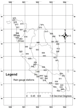
Figure 1 Geographical map of the Peninsular Malaysia with the rainfall stations considered

3.2 Extreme rainfall Indices Calculation

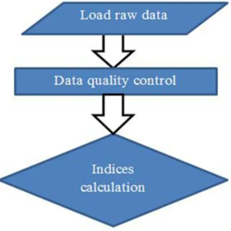
determining climatic indices. The RClimdex software performs the following procedure:

Figure 2 RClimDex climate indices calculation stages

The RClimDex QC performs the following procedure:

• Replace all missing values (currently coded as -99.9) into an internal format that R recognizes (i.e. NA, not available),

• Replace all unreasonable values into NA. Those values include daily precipitation amounts less than zero, daily maximum temperature less than the daily minimum temperature.

1081

Table 1: List of 8 selected ETCCDMI Extreme Rainfall Indices

ID Indicator name Definition Unit

R10 Frequency of

heavy precipitation days

Annual count of days when PRCP>=10mm mm

R20 Frequency of

very heavy precipitation

Annual count of days when PRCP>=20mm mm

R30 Frequency of

extremely heavy precipitation

Annual count of days when PRCP>=30mm mm

SDII Simple daily

intensity index

Let RR_wj be the daily precipitation amount

on wet days, where w(RR ≥ 1mm), in period j. If W is the number of wet days during

period j, then:

1( ) /

W

j _w wj

SDII

mm/da y

CWD Consecutive wet

days

Let RR_ij be the daily precipitation amount

on day i during period j. Count the largest

number of consecutive days where: RR_ij≥

1mm

Days

R95p Very wet days _Let

wj

RR be the daily precipitation amount

on a wet day w (RR ≥ 1mm) during time

period i, and let RR_wn95 be the 95th percentile of precipitation on wet days during the comparison period of climate base. Let W be the number of wet days during this period, then:

1

95_Pj W _wj

w

R RR

95

wj wn

RR RR

mm

R99p Extreme wet

days

Let RR_wj be the daily precipitation amount

on a wet day w (RR ≥ 1mm) during time

period i, and let RR_wn99 be the 99th

percentile of precipitation on wet days during the comparison period of climate

base. Let W be the number of wet days during this period, then:

1

99_Pj W _wj

w

R

99

wj wn

RR RR

PRCPTOT Annual total wet-day

precipitation

Let RR_ij be the daily precipitation amount

on day i in period j. If I represent the number of days in j, then:

1( )

J

j i ij

PRCPTOT RR

mm

3.3 Spatial Dependence

Kriging uses semivariance to measure the spatially correlated component, a component that is also called spatial dependence or spatial autocorrelation which expresses the spatial dependence between neighboring observations. The semivariogram quantifies the relationship between the semivariance and the distance between sampling pairs. A semivariogram, plots the average semivariance against the average distance, this function may be used alone as a measure of spatial autocorrelation [31].The semivariance is computed by:

2 1 2 1 ( ) [ ( ) ( )] n i j n i

h z s z s h

where ( )h is the average semivariance between known points, s_i and s_j

separated by distanceh; n is the number of pairs of sample points sorted by direction in the bin; and zis the attribute value. Semivariogram is modeled by

fitting a theoretical function such as: Spherical, Exponential, Gaussian orLinear

models to ensure that the solution is unbiased and has minimum variance.

1083 2

1

1

ˆ

{[ ( ) ( )] / 0

n

i i i

n i

MEE z s z s

where z s( )_i is the measured value of regional value (ReV) at the location si,

ˆ( )_i

z s is the estimated value of ReV at the location si, _i is the calculated

Kriging estimation error variance for ˆ( )z s_i , and n is the number of estimated

values. On the other hand, the root mean square error (RMSE) is close to one as follows:

1 2 2

1_{{( ( ) ˆ( )) / ] } 1}

i i i

n

RMSE z s z s .

After a suitable semivariogram model fitting and its parameter estimations, the Kriging technique is applied to estimate the value of a variable at every grid point, where no observation is available.

3.4 Ordinary Kriging

Ordinary Kriging (OK) is a geostatistical technique to modelling. OK relies on the spatial correlation structure of the data in determining the weighting values. This is a more rigorous approach to modelling, as correlation between data points determines the estimated value at an unsampled point. The semivariograms provides estimated values of the correlation structure for a finite number of distances. In performing OK, semivariogram values for any distance are required. The kriging estimators are but variants of the basic linear regression

estimator Z u*( ) defined as [33]:

( ) *

1

( ) ( ) [ ( ) ( )]

n u

Z u m u Z u m u

with uand u: location vectors for estimation point and one of the neighbouring

data points, indexed by , where n u( )is the number of data points in local

neighbourhood used for estimation of Z u*( ), m u( )and m u( ) are the expected

values of Z u( ) and Z u( )respectively, ( )u is the Kriging weight assigned to

datum z u( )for estimation location u; same datum will receive different weight

for different estimation location. Z u( ) is treated as a random field with a trend

Kriging estimates residual at u as weighted sum of residuals at surrounding data points. The Kriging weights , are derived from covariance

function or semivariogram.

The main goal of (Eq. 1) is to determine weights that minimize the

variance of the estimator: _E2( )u Var Z u{ *( )Z u( )} , under the unbiased

constraint E Z u{ *( )Z u( )} 0 .

The random field Z u( ) is decomposed into residual and trend components given

as:

( ) ( ) ( )

Z u u m u ,

with the residual component treated as a field with a stationary mean 0 and a stationary covariance (a function of lag h, but not of position, u):

{ ( )} 0

E u

( ( ), ( )} ( ( ) ( )} ( )

Cov u u h E u u h C h

The residual covariance function is generally derived from the input semivariogram model:

( ) (0) ( ) ( )

C h C h Sill h .

In ordinary Kriging, rather than assuming that the mean is constant over the entire domain, following [34] it is assumed that it is constant in the local neighbourhood of each estimation point that ism u( )m u( )for each nearby data

valuez u( ) used in estimatingZ u( ). In this case, the Kriging estimator can be

written in the following form:

( ) *

1

( ) ( ) ( )[ ( ) ( )]

n u

Z u m u u Z u m u

( ) ( )

1 1

( ) ( ) 1 ( ) ( )

n u n u

u Z u u m u

Filtering the unknown local mean by requiring that the Kriging weights sum to 1, leading to an ordinary kriging estimator [21];

( ) * 1 ( ) ( ) ( ) n u OK OK

Z u u Z u

with

( )

1

( ) 1

1085

3.0 RESULTS AND DISCUSSIONS

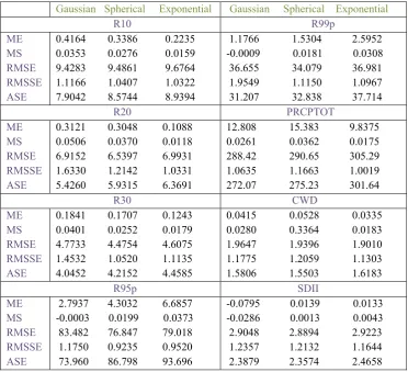
The daily rainfall data sets of 75 rain-gauge stations across peninsular Malaysia for the period January 1975 to November 2008 were used to calculate the rainfall indices selected in this study given (Table 1). The first important step in performing OK is modelling the spatial dependence through either of the semivariogram models. A semivariogram is an important function to indicate spatial correlation in observations measured at sample locations. Three semivariogram models such as: Gaussian, Spherical and Exponential were employed in this study. The cross validation result from the fitted models is given (Table 2).

Table 2: Summary results for cross validation of semivariogram models

Gaussian Spherical Exponential Gaussian Spherical Exponential

R10 R99p ME

MS RMSE RMSSE ASE

0.4164 0.3386 0.2235 0.0353 0.0276 0.0159 9.4283 9.4861 9.6764 1.1166 1.0407 1.0322 7.9042 8.5744 8.9394

1.1766 1.5304 2.5952 -0.0009 0.0181 0.0308 36.655 34.079 36.981 1.9549 1.1150 1.0967 31.207 32.838 37.714

R20 PRCPTOT ME

MS RMSE RMSSE ASE

0.3121 0.3048 0.1088 0.0506 0.0370 0.0118 6.9152 6.5397 6.9931 1.6330 1.2142 1.0331 5.4260 5.9315 6.3691

12.808 15.383 9.8375 0.0261 0.0362 0.0175 288.42 290.65 305.29 1.0635 1.1663 1.0019 272.07 275.23 301.64

R30 CWD ME

MS RMSE RMSSE ASE

0.1841 0.1707 0.1243 0.0401 0.0252 0.0179 4.7733 4.4754 4.6075 1.4532 1.0520 1.1135 4.0452 4.2152 4.4585

0.0415 0.0528 0.0335 0.0280 0.3364 0.0183 1.9647 1.9396 1.9010 1.1775 1.2059 1.1303 1.5806 1.5503 1.6183

R95p SDII ME

MS RMSE RMSSE ASE

2.7937 4.3032 6.6857 -0.0003 0.0199 0.0373 83.482 76.847 79.018 1.1750 0.9235 0.9520 73.960 86.798 93.696

The cross validation, is used to find the best model among the competing models. The goal is to have standardized mean prediction errors near 0, small squared prediction errors, average standard error near root-mean-squared prediction errors, and standardized root-mean-root-mean-squared prediction errors near 1 (ArcGis Desktop 10). From (Table. 2) it can be seen that the Exponential semivariogram model best fits the data sets, therefore, is chosen as the best model for the spatial interpolation.

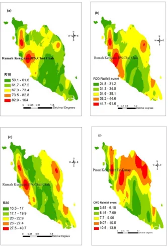
According to the previous analysis, the exponential semivariogram model is chosen to realize the OK interpolation using the eight adapted rainfall events. The OK is used to estimate the spatial pattern of the representative precipitation indices, producing one map for each index. The climatological pattern of the indices over the peninsular Malaysia indicates some areas that recorded low and high values for both the frequency and intensity indicators.

1087

1089

4.0 SUMMARYANDCONCLUSION

The main objective of this work is to analyse the spatial patterns of eight rainfall indices in peninsular Malaysia in identifying areas that are more related to risk of extreme rainfall event. First, the indices were calculated from the daily rainfall data sets using RClimDex. The indices were grouped into two: The first group calculates the frequency of the event exceeding a defined threshold (CWD, R10mm, R20mm and R30). The second group measures the precipitation depth or intensity (PRCPTOT, SDII, R95P and R99P). Based on the results in this work, the following conclusions were made:

1. The Chui Chak station realised the most extremely rainfall events based on the indices R10, R20 and R30. Moreover, it has also being identified as the area with the highest annual total precipitation in wet days (PRCPTOT). This is not surprising, as aforementioned, IPCC [27] reported that “wet extremes are projected to become more severe in many areas where mean precipitation is expected to increase”, this is in line with the findings [35] “Based on the values of descriptive statistics, the five highest mean rainfall amounts among the stations are Chui Chak (W10), followed by Kg Menerong (E06), Endau (E13), …”.

2. Kg Menerong station realised the highest value for the indices that measure heavy precipitation that exceeds the 95 and 99 percentile thresholds, expressed by the 95th and 99th percentiles (R95p and R99p) indices.

3. Pusat Kesihatan Bt.Kurau is the station identified with the highest CWD precipitation.

4. Pintu Kawalan Tampok Batu Pahat is the station with highest SDII.

The CWD, PRCPTOT and SDII are not necessarily associated with climate extremes but provide useful information about the relationship between changes in extreme conditions and other aspects of the distribution of the daily precipitation [36]. Finally, the Kg Menerong and Chui Chak are the areas identified that are more related to risk of extreme rainfall events. Therefore, we strongly recommend that researchers should give more attention to the identified areas in knowing the dynamics of the rainfall data generating the extreme events.

REFERENCES

[1] Durao, R., Pereira, M.J., Costa, A.C., Corte-Rea, J.M. and Soares, A. 2009. Indices of precipitation extremes in Southern Portugal – a geostatistical approach. Nat. Hazards Earth Syst. Sci., 9, 241–250, 2009 www.nat-hazards-earth-syst-sci.net/9/241/2009/

[2] Radinovic, D. & Curic, M. 2009. “Deficit and surplus of precipitation as a continuous function of time”. Theor. Appl. Climatol., doi:10.1007/s00704-009-0104-2.

[3] Karagiannidis, A., Karacostas, T., Maheras, P. & Makrogiannis, T. 2009. “Trends and seasonality of extreme precipitation characteristics related to mid-latitude cyclones in Europe”. Adv. Geosci., 20, 39–43. www.adv-geosci.net/20/39/2009.

[4] Guhathakurta, P., Sreejith, O. P. & Menon, P. A. 2011. “Impact of climate change on extreme rainfall events and flood risk in India”. Journal of Earth System Science, Volume 120, Issue 3, 359-373.

[5] Brooks, H.E. & Stensrud, D. J. 2000. “Climatology of Heavy Rain Events in the United States from Hourly Precipitation Observations”. Monthly Weather Review, 128(22), 1194 – 1201.

[6] Hayhoe, K., Wake, C. P., Huntington, T. G., Luo, L., Schwarz, M. D., Sheffield, J., Wood, E., Anderson, B., Bradbury, J., DeGaetano, A., Troy, T. J. & Wolfe, D. 2007. “Past and future changes in climate and hydrological indicators in the US Northeast”. Climate Dynamics 28: 381-407.

[7] Groisman, P. Y., Richard, W. K., David, R. E., Thomas, R. K., Gabriele, C. H. & Vyacheslav N. R. 2005. “Trends in Intense Precipitation in the Climate Record”. J. Climate, 18, 1326–1350. doi: http://dx.doi.org/10.1175/JCLI3339.1

[8] Schumacher, R..S. & Johnson, R.H. 2005. Organization and

Environmental Properties of Extreme-Rain-Producing Mesoscale Convective Systems. Amer. Met. Soc., 133, 961-976.

1091

New England and Clean Air-Cool Planet, http//: CarbonSolutionsNE.org, (Last access date: 21/02/2013).

[10] Klein Tank, A.M.G., Francis, W. Z. and Xuebin, Z. 2009. “Guidelines on Analysis of extremes in a changing climate in support of informed decisions for adaptation”. Climate Data and Monitoring, WCDMP-No. 72.

[11] Wan Zawiah, W. Z., Abdul Aziz, J. and Kamarulzaman, I. 2012. Bayesian Change point Analysis of the Extreme Rainfall Events. Journal of Mathematics and Statistics 8 (1): 85-91, 2012

[12] Syafrina, A. H., Zalina, M. D. & Juneng, L. 2012. A Spatial Analysis of Hourly Extreme Rainfall Patterns in Peninsular Malaysia. www.jba.gov.my/.../174-a-spatial-analysis-of-hourly-extreme-rainfall..., (Last access date: 13/02/2013).

[13] Diong, J. Y., Subramaniam M., Munirah A. & Siva S. G. 2011. “ Trends in intensity & frequency of precipitation extremes in Malaysia from 1951

to 2009”. http://www.wcrpclimate.org/conference2011/posters/C23/C23_JeongYik

_T227A.pdf.

[14] Zalina MD, Amir HMK, Mohd NMD, Van-Thanh VN (2002) Statistical

analysis of at-site extreme rainfall processes in Peninsular Malaysia. Proceedings of the Fourth International FRIEND Conference held at Cape Town. South Africa. March 2002. IAHS Publ. no. 274. 61-68

[15] Juneng, L., Tangang, F.T. and Reason, C.J.C. 2007. Numerical case study of an extreme rainfall event during 9–11 December 2004 over the east coast of Peninsular Malaysia. Meteorol Atmos Phys, 98, 81–98, DOI 10.1007/s00703-006-0236-1.

[17] Annazirin, E., Mar dhiyyah, S. & Wan Zawawiah W. Z. 2012. Preliminary Study on Bayesian Extreme Rainfall Analysis: A Case Study of Alor Setar, Kedah, Malaysia. Sains Malaysiana, 41(11),1403–1410. [18] Klein Tank, A.M.G. & Konnen, G.P. 2003. Trends in indices of daily

temperature and precipitation extremes in Europe, 1946–99. Journal of Climate, 16:22, 3665–3680.

[20] Mair, A and Fares, A. 2011. Comparison of Rainfall Interpolation Methods in a Mountainous Region of a Tropical Island. Journal of Hydrologic Engineering, Vol. 16, No. 4, 371-383.

[21] Goovaerts, P. 2000: Geostatistical approaches for incorporation elevation into the spatial interpolation of rainfall, J. Hydrol., 228, 113–129.

[22] Schuurmans, J.M., Bierkens, M. F. P. & Pebesma, E. J. 2007. Automatic Prediction of High-Resolution Daily Rainfall Fields for Multiple Extents: The Potential of Operational Radar. Journal of hydrometeorology, vol. 8, 1204-1224. DOI: 10.1175/2007JHM792.1.

[23] Krahenmann, S. and Ahrens, B. 2010. On daily interpolation of precipitation backed with secondary information. Adv. Sci. Res., 4, 29– 35, 2010. www.adv-sci-res.net/4/29/2010/.

[24] Yang, T., Shao, Q., Hao, Z-C., Chen, X., Zhang, Z., Xu, C-Y. & Sun, L. 2010. “Regional frequency analysis and spatio-temporal pattern characterization of rainfall extremes in the Pearl River Basin, China”. J Hydrol 380:386–405. doi:10.1016/j.jhydrol.2009.11.013.

[25] Suhaila, J. & Abdul Aziz, J. 2011a. “Spatial analysis of daily rainfall intensity and concentration index in Peninsular Malaysia”. Theor Appl Climatol (2012). 108:235–245. DOI 10.1007/s00704-011-0529-2.

[26] Wong CL, Venneker R, Uhlenbrook S, Jamil ABM, Zhou Y (2009) Variability of rainfall in Peninsular Malaysia. Hydrol Earth Syst Sci Discuss 6:5471–5503, www.hydrol-earth-syst-sci-discuss.net/ 6/5471/2009/

[27] IPCC, 2007. “Climate Change 2007:The Physical Science Basis”. Contribution of Working Group 1 to the Fourth Assessment Report of the Intergovernmental Panel on Climate Change. Cambridge University Press, Cambridge, UK, NY, USA, 1009pp.

[28] Wan Azli, W. H. 2010. Influence of Climate Change on Malaysia’s Weather Pattern. Malaysia Green Forum 2010 (MGF2010) Seri Siantan Conference Hall, Perbadanan Putrajaya, 26-27 April 2010.

[29] Zhang, X. & Yang, F. 2004. “RClimDex (1.0) User Guide”. Climate Research Branch Environment Canada Downsview, Ontario Canada, 1-22. http://precis.metoffice.com/Tutorials/RClimDexUserManual.doc. [30] Haylock, M. R., Peterson, T. C., Alves, L. M., Ambrizzi, T.,

1093

M. Coronel, G., Corradi, V., Garcia, V. J., Grimm, A. M., Karoly, D., Marengo, J. A., Marino, M. B., Moncunill, D. F., Nechet, D., Quintana, J., Rebello, E., Rusticucci, M., Santos, J. L., Trebejo, I. & Vincent, L. A. 2006. “Trends in total and extreme South American rainfall 1960-2000 and links with sea surface temperature”. Journal of Climate. 19, 1490-1512.

[31] Kang, T. C. 2012. “Introduction to Geographic Information Systems”. Six edition, McGRAW HILL International Edition, 314-338, Singapore. [32] Clark, I. & Harper, W. 2000. “Practical Geostatistics 2000”. Ecosse

North America Lic, Columbus, Ohio, USA.

[33] Goovaerts, P., 1997. Geostatistics for Natural Resources Evaluation. Oxford Univ. Press, New York, 512 pp.

[34] Geoff, B. 2005. KRIGING. C&PE 940, 19 October 2005, people.ku.edu/~gbohling/cpe940/Kriging.pdf, (Last access date: 02/02/2013).

[35] Suhaila, J., Ching-Yee, K., Fadhilah, Y. and Hui-Mean, F. 2011b. Introducing the mixed distribution in fitting rainfall data. Open J Mod

Hydrol, 1(2):11–22. doi:10.4236/ojmh.2011.12002, http://www.SciRP.org/journal/ojmh

Appendix

Stations code and name

1 PINTU A.BAGAN,AIR ITAM 40 Tangkak

2 ARAU 41 Malacca

3 S. K. KG. AUR GADING 42 Mersing

4 LDG. BATU KAWAN 43 Hospital Port Dickson

5 LDG. BKT. ASAHAN 44 Endau

6 KG. CHEBONG 45 Setor JPS Sikamat Seremban

7 GUAR NANGKA 46 Sg.Lui Halt

8 KLINIK BIDAN ,JAMBU BONGKOK 47 Petaling Jaya

9 JANDA BAIK 48 Subang

10 JAM. SG. SIMPANGN ,JLN. EMPAT 49 Empangan Genting Kelang

11 IBU BEKALAN KAHANG , KLUANG 50 Gombak

12 KAKI BUKIT 51 Rumah Pam Pahang Tua,Pekan

13 SEK. KEB. KEMASEK 52 Kuantan

14 SEK. KEB. KG. JABI 53 Rumah Pam Paya Kangsar

15 LDG. KIAN HOE , KLUANG 54 Rumah Kerajaan JPS,Chui Chak

16 KODIANG 55 Sitiawan

17 DISPENSARI KROH 56 JPS Kemaman

18

STN. PEMEREKSAAN HUTAN

,LAWIN 57 Ldg Boh

19 PEKAN MERLIMAU 58 Ipoh

20

RUMAH PENJAGA JPS. PARIT

NIBONG 59 Sek.Men. Sultan Omar, Dungun

21 PENDANG 60 Gua Musang

22 JPS. WILAYAH PERSEKUTU 61 Kg. Menerong

23 LDG. GETAH KUKUP , PONTIAN 62 Pusat Kesihatan Bt.Kurau

24 LDG. BENUT ,RENGAM 63 Rumah JPS, Alor Pongsu

25 LDG. SG. SABALING 64 Selama

26 GENTING SEMPAH 65 Stor JPS Kuala Trengganu

27 LDG. SENGKANG 66 Bkt Berapit

28 KG. MERANG ,SETIU 67 Kolam Takongan Air Itam

29 IBU BEKALAN SG. BERNAM 68 Klinik Bkt. Bendera

30 KG. SG. TUA 69 Rumah Pam Bumbong Lima

1095

32 Stor JPS Johor Bahru 71 Kota Bharu

33 Pintu Kawalan Tampok Batu Pahat 72 Alor Star

34 Senai 73 Ampang Pedu

35 Sek.Men.Bkt Besar di Kota Tinggi 74 Padang Katong ,Kangar

36 Sek.Men.Inggeris Batu Pahat 75 Abi Kg. Bahru

37 Pintu Kawalan Sembrong