Bayesian Methods for Images and Trees

(1)

ABSTRACT

LI, MENG. Bayesian Methods for Images and Trees. (Under the direction of Subhashis Ghoshal.)

Images (2D, 3D, or even conceptually higher dimensional) are a fundamental data type and arise frequently in many areas such as neuroscience, astronomy, engineering and en-vironmental science. Denoising and boundary detection are among problems of long-standing interest. In the first part of the dissertation, we propose a multiscale model for Gaussian noised images under a Bayesian framework for both 2-dimensional (2D) and 3-dimensional (3D) images. We use a Chinese restaurant process prior to randomly gener-ate ties among intensity values at neighboring pixels in the image. The resulting Bayesian estimator enjoys some desirable asymptotic properties for identifying precise structures in the image. The proposed Bayesian denoising procedure is completely data-driven. A conditional conjugacy property allows analytical computation of the posterior distribu-tion without involving Markov chain Monte Carlo (MCMC) methods, making the method computationally efficient. Simulations on Shepp-Logan phantom and Lena test images confirm that our smoothing method is comparable with the best available methods for light noise and outperforms them for heavier noise both visually and numerically. The proposed method is further extended for 3D images. A simulation study shows that the proposed method is numerically better than most existing denoising approaches for 3D images. A 3D Shepp-Logan phantom image is used to demonstrate the visual and numer-ical performance of the proposed method, along with the computational time. MATLAB toolboxes are made available online (both 2D and 3D) to implement the proposed method and reproduce the numerical results.

Translation Invariant (TI) cycle spinning is an effective method for removing artifacts from images. However, for a method usingO(n)time, the exact TI cycle spinning by aver-aging all possible circulant shifts requiresO(n2₎_{time where}_n_{is the number of pixels, and}

(2)

mul-tiscale approaches. In the second part of the dissertation, we propose a Fast Translation Invariant (FTI) algorithm and a more generalk-Translation-Invariant (k-TI) algorithm al-lowing TI for the lastk scales of the image, which are applicable to generald-dimensional images (d =2, 3, . . .) with either Gaussian or Poisson noise. The proposed FTI leads to the exact TI estimation but only requiresO(nlog₂n)time. The proposedk-TI can achieve al-most the same performance as the exact TI estimation, but requires even less time. We achieve this by exploiting the regularity present in the multiscale structure, which is jus-tified theoretically. The proposed FTI andk-TI are generic in that they are applicable on any smoothing techniques based on the multiscale structure. We demonstrate the FTI and k-TI algorithms on some recently proposed state-of-the-art methods for both Poisson and Gaussian noised images. Both simulations and real data application confirm the appeal-ing performance of the proposed algorithms. Matlab toolboxes are online accessible to reproduce the results and be implemented for general multiscale denoising approaches provided by the users.

Detecting boundary of an image based on noisy observations is a fundamental prob-lem of image processing and image segmentation. For a d-dimensional image (d = 2, 3, . . .), the boundary can often be described by a closed smooth (d −1)-dimensional manifold. In the third part of the dissertation, we propose a nonparametric Bayesian ap-proach based on priors indexed bySd−1, the unit sphere inRd. We derive optimal poste-rior contraction rates using Gaussian processes or finite random series pposte-riors using basis functions such as trigonometric polynomials for 2-dimensional images and spherical har-monics for 3-dimensional images. For 2-dimensional images, we show a rescaled squared exponential Gaussian process onS1achieves four goals of guaranteed geometric restric-tion, (nearly) minimax optimal rate adaptive to the smoothness level, convenient for joint inference and computational efficiency. We conduct an extensive study of its reproducing kernel Hilbert space, which may be of interest by its own and can also be used in other con-texts. Several new estimates on the modified Bessel functions of the first kind are given. Simulations confirm excellent performance of the proposed method and indicate its ro-bustness under model misspecification at least under the simulation settings.

(3)

(4)

c

(5)

Bayesian Methods for Images and Trees

by Meng Li

A dissertation submitted to the Graduate Faculty of North Carolina State University

in partial fulfillment of the requirements for the Degree of

Doctor of Philosophy

Statistics

Raleigh, North Carolina 2015

APPROVED BY:

David B. Dunson Armin Schwartzman

Hua Zhou Subhashis Ghoshal

(6)

DEDICATION

(7)

BIOGRAPHY

(8)

ACKNOWLEDGEMENTS

To begin with, I would like to express my deepest gratitude to my advisor Dr. Subhashis Ghoshal for his continued supports and great mentoring. His patience, passion towards academics and tremendous work ethics never fail to surprise me. He sets a good example for me to stay persistent beyond the wall of research. His caring and unique sense of humor make it a great experience to work with him.

I would also like to extend my appreciation to my committee members, Dr. David Dun-son, Dr. Armin Schwartzman and Dr. Hua Zhou, for their supports and insightful com-ments. They have always been very generous for their valuable time and energy during this entire process. I also thank Dr. Aziz Amoozegar for kindly serving on my committee as the graduate school representative.

I would like to sincerely thank professors at NC State. I am especially thankful to Dr. Ana-Maria Staicu and Dr. Howard Bondell with whom I worked for my first research project on functional data analysis. I offer much thanks to Dr. Armin Schwartman from whom I have learned a lot about PET images and numerous tricks to display figures in LA_TEX.

I also thank Dr. Sujit Ghosh who served as the DGP providing invaluable suggestions and is always there to help. Thank Dr. Hua Zhou and Dr. Eric Laber for the amazing advanced computing course. Thank Dr. Dennis Boos for the great course on advanced inference. I also thank all the fantastic staff in the department, Terry Byron, Chris Waddell, Adrian Blue, Alison McCoy and Lanakila Alexander, for their great service to the department.

I thank Professor Aad van der Vaart for many helpful discussions and pointing out im-portant references for the boundary detection problem.

My appreciation goes to MaxPoint where I interned last summer. Thank my former colleagues Mark Lowe, Satish Anjilvel, Jianling Zhong and Zhen Han.

Thank all my friends and fellow students at NC State. To Peng, Anran, Shikai, Brad, Bo, Christ, Hao and many others: thank you!

(9)

LIST OF TABLES

Table 2.1 Illustration of the corresponding constraint matrixAand prior prob-ability P(_{C |}M)for given configuration_C. The column of_C contains all possible configurations belonging to the same tie structures, while the diagonally tied ones are crossed out. The constraint matrix Ais for the first_C, while the other constraint matrices can be obtained by permuting the columns ofAaccording to the tieing structures. The last column is the prior probability P(_{C |}M), which is shared by all configurations in the same category. . . 15 Table 2.2 Numerical comparison of smoothing methods for the phantom

im-age when noise standard deviationσ=0.1. The mean MSE (_×10−2₎_,

MAD (_×10−2₎_{and HD (}_×₁₀−2₎ _{of 100 simulations are reported. The}

maximum standard error for each criterion is given by the last row. All methods except TI-Haar and Bayesian dictionary learning use 121 local shifts to remove artifacts. The running time for each local shift and the total time are reported in the last two columns. . . 22 Table 2.3 Numerical comparison of smoothing methods for the Lena image at

various noise levels in terms of MSE (_×10−2_{). 100 simulations are run}

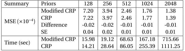
and the maximum standard errors are given by the last row. All meth-ods except TI-Haar and Bayesian dictionary learning use 121 local shifts to remove artifacts. The running time for each local shift and the total time whenσ=0.2 are reported; the running time is similar for the other noise levels. . . 26 Table 2.4 Comparison of the modified CRP prior and the CRP prior using noisy

phantom images with the standard deviation σ = 0.1 and a con-stant background noise 0.01 for various image sizes. We report the MSE(_×10−4_{) for each of them, the differences (modified CRP}₋_CRP)

and the standard errors of the differences. The time taken by each prior is reported by the last two rows. The results are based on 121 local shifts and 100 simulations. . . 26 Table 2.5 Scalability of the Bayesian CRP using noisy phantom images with the

standard deviationσ = 0.1 and a constant background noise 0.01. The result is based on 121 local shifts and 100 simulations. . . 27 Table 2.6 3D denoising for two imagesf1, f2in terms of MSE(×10−2). Bayesian

CRP (the first row) uses 5×5×5 local shifts and is based on 100 replica-tions. The mean of 100 MSEs is reported. The maximum standard er-ror for each column is reported in the last row. The numerical records for the other five methods to estimate f1and f2are from Mukherjee

(12)

Table 2.7 Numerical performance of the Bayesian CRP on the 3D Shepp-Logan phantoms. The mean MSEs and average computational times are re-ported. The average computational time includes the Optimization time to select the smoothing parametersM andτ, Estimation time per shift given the selected smoothing parameters, and the Total time when using 5_×5_×5 local shifts. The total time=the optimization time

+the estimation time per shift×the number of shifts. 100 simula-tions are run and the standard errors of MSEs are given in the paren-theses. Results are obtained without using any parallel computing techniques. . . 34 Table 3.1 Summary of computing time for a general operatorG applied on the

imageX which hasn pixels. . . 55 Table 3.2 Performance on test images (Gaussian noise). The 5 columns are

im-ages, MSE of the 0-TI estimate, MSE and percentage reduced (com-pared to the 0-TI) of the FTI, selectedk and percentage reduced of MSE (compared to the 0-TI) of thek-TI. Results are obtained by aver-aging 100 simulations except for the selectedk which uses the mode.

. . . 61 Table 4.1 Lebesgue errors (_×10−2_{) of the methods based on 100 simulations.}

The standard errors are reported below in the parentheses. . . 85 Table 4.2 Performance of the methods for Gaussian noised images based on

100 simulations. The Lebesgue error between the estimated bound-ary the true boundbound-ary is presented. The maximum standard errors of each column are reported in the last row. . . 89 Table 5.1 Summary of the parameter estimates in Model 5.1. The first two rows

are the posterior means forβand the diagonal elements ofΣ. The 3rd and 4th rows are the lower and upper bound of a 95% credible sets forβ. The 5th row is the percentage ofβ_i’s that the corresponding coefficient is significant using a 95% credible set. . . 106 Table A.1 Developed Matlab toolboxes or R packages and the corresponding

(13)

LIST OF FIGURES

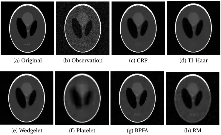
Figure 2.1 Comparison of the Bayesian smoothing method with other ap-proaches for the 256_×256 Shepp-Logan phantom shown in (a). The noisy observation with standard deviationσ =0.1 and a constant background noise 0.01 is shown in (b). The six denoising methods (c)–(h) are respectively Bayesian CRP, TI-Haar, wedgelet, platelet, Bayesian dictionary learning and running median. All methods ex-cept TI-Haar and Bayesian dictionary learning use 121=11_×11 local shifts to remove artifacts. . . 23 Figure 2.2 Comparison of the Bayesian smoothing method with other

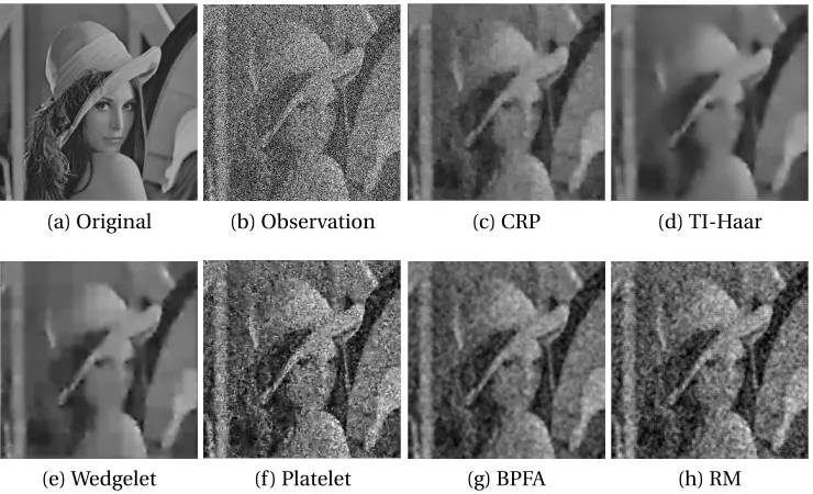
ap-proaches for the 512_×512 Lena image shown in (a). The noisy ob-servation with standard deviationσ =0.1 is shown in (b). The six denoising methods (c)–(h) are respectively Bayesian CRP, TI-Haar, wedgelet, platelet, Bayesian dictionary learning and running me-dian. All methods except TI-Haar and Bayesian dictionary learning use 121=11_×11 local shifts to remove artifacts. . . 24 Figure 2.3 Comparison of the Bayesian smoothing method with other

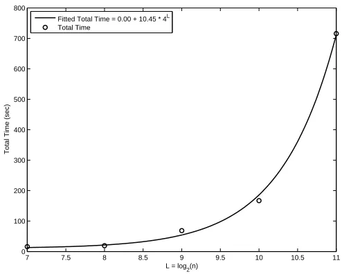
ap-proaches for the 512_×512 Lena image shown in (a). The noisy ob-servation with standard deviationσ =0.6 is shown in (b). The six denoising methods (c)–(h) are respectively Bayesian CRP, TI-Haar, wedgelet, platelet, Bayesian dictionary learning and running me-dian. All methods except TI-Haar and Bayesian dictionary learning use 121=11×11 local shifts to remove artifacts. . . 24 Figure 2.4 Scalability of the Bayesian CRP. We plot the total time with the

num-ber of levelsL =log₂(n), and fit a straight line when the number of pixelsn2₌₄L _{is the predictor. The fitted line is: Total Time}₌_0.00₊ 10.45n2_{thus linear in the total number of pixels. . . .} ₂₇

(14)

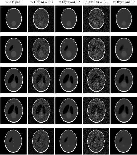
Figure 2.6 Performance of the Bayesian CRP approach for a 3D Shepp-Logan phantom image (n=128). Each row corresponds to a cross-section of the image; the five rows are the 40th, 50th, 60th, 65th and 80th slice, and are selected to represent various features of a typical phan-tom image. The first column is the original image. Then 2nd col-umn is the noisy observation with noise level 0.1, followed by the smoothed version in the 3rd column. The 4th and 5th column are the noisy observation and the smoothed image when the noise level is 0.2. Here the Bayesian CRP approach uses 5_×5_×5 local shifts. . . . 33 Figure 3.1 Smoothed images applying the FTI algorithm. The first row is for

the phantom image (size 512) with Gaussian noise and the second row is for the Saturn image (size 256) with Poisson noise. The four columns are the true image, observation, 0-TI and Full TI estimates respectively. . . 57 Figure 3.2 Performances of the k-TI algorithm using phantom images with

Gaussian noise (2D image with size 512 and 3D image with size 128) and the Saturn image with Poisson noise(2D image with size 256). Thex-axis is the TI levelkand they-axis is the MSE (the first row) or the Time (the second row). The maximumk in each subplot means the Full TI estimation. For plots in the second row, the red line with-out markers is for the naive TI approach and the blue line with mark-ers for the proposed Fast TI algorithm. All results are based on 100 simulations. . . 58 Figure 3.3 Effectiveness plot on the phantom test image (size 512) with

Gaus-sian noise (standard deviation 0.1). The pairs(k,E(L−k))are plotted whereE(L−k)is calculated using the 2-norm on a matrix. . . 59 Figure 3.4 Performance of the FTI operator on test images with Gaussian noise

(from left to right, top to bottom: Barbara, boat, fingerprint, flin-stones, house, lena, man, mandrill, parrot, and peppers). We plot the observation, 0-TI and Full TI estimates for each image. . . 60 Figure 3.5 Effect ofk-TI algorithms when applying Bayesian CRP on the

Chan-dra image. (a) is a single spectral channel (the 66th) , while (b) is the average across all 256 channels. (c) and (d) are the smoothed single spectral channel images using 0-TI and the Full TI algorithm. . . 61 Figure 4.1 Decay rate of the eigenvalues of the squared exponential kernel.

(15)

Figure 4.2 Performance on binary images (Column 1) with elliptic boundary. Column 2–4 plot the estimate (solid line in red) against the true boundary (dotted line in black). A 95% uniform credible band (in gray) is provided for the Bayesian estimate (Column 2). . . 86 Figure 4.3 Performance on binary images (Column 1) when the boundary

curve is an regular triangle. Column 2–4 plot the estimate (solid line in red) against the true boundary (dotted line in black). A 95% uni-form credible band (in gray) is provided for the Bayesian estimate (Column 2). . . 87 Figure 4.4 Proposed Bayesian estimates for Gaussian noised images with

ellip-tic boundary. Plots (a)–(d) are the noisy observations. Figures (e)– (h) are the corresponding estimates (solid line in red) against the true boundary (dotted line in black), with a 95% uniform credible band (in gray). . . 89 Figure 5.1 The plot on the left is blood arteries of one subject, where the colors

indicate the regions in the brain: Front (red), Back (gold), Left (cyan), Right (blue). The plot on the right is the corresponding binary tree representation from the back tree. . . 102 Figure 5.2 Demonstration of the breadth-first index and complete-binary-tree

index (label). The 6th and 7th node (left panel) is indexed as 8 and 9 respectively using the complete-binary-tree index (right panel). . . . 103 Figure 5.3 Original data set of one subject. The left panel is for the thickness

while the right one is for the branch length. The x-axis is the breadth-first index of each node. . . 107 Figure 5.4 Trend of thinkness and branch length with respect to the depth. The

left panel is for the thickness while the right one is for the branch length. The x-axis is the depth level. . . 108 Figure 5.5 Data after pre-procesing. The left panel is for the thickness while

(16)

Chapter 1 Introduction

1.1 Background

Data sets of complex objects have attracted a lot of attention over the last two decades in literature due to rapid advancement of technology and development of statistical analysis tools, and play a critical role in the so-called “age of big data". For example, they may include functional data or curves (Ramsay and Silverman, 2002, 2005), images (Qiu, 2005; Sonka et al., 2014), trees (Shen, 2012), shapes (Dryden and Mardia, 1998; da Fontoura Costa and Cesar Jr, 2010) and many others such as graphs and networks, just to name a few. The corresponding analysis is challenging since the data structure is complex or the data size or number of covariates is extremely large (largenlargepor largepsmalln). For instance, images (especially 3-dimensional) typically have extremely large number of observations and the tree space could be highly non-Euclidean.

(17)

which avoids cross-validation type tuning often used in non-Bayesian approaches. It also leads to convenient inference by the corresponding posterior distributions and provides a tractable way to fully quantify uncertainty in the analysis.

In this dissertation, we shall focus on analyzing image and tree data sets, and de-velop computationally efficient statistical methods with desirable theoretical properties for complex data types. The mentioned advantages and convenience of the Bayesian ap-proach will be exemplified in the later chapters.

1.2 Bayesian multiscale image denoising

Images (2D, 3D, or even conceptually higher dimensional) are a fundamental data type and arise frequently in many areas such as neuroscience, astronomy, engineering and environ-mental science. Image denoising is among problems of longstanding interest particularly for satellite images, photon-limited images in astronomy and biomedical images such as Positron emission tomography (PET) scans, just to name a few.

An observed 2-dimensional (2D) image can be viewed as a two-dimensional data ma-trix X = ((X₍j,k))), where j,k = 1, . . . ,n, as the sum of the underlying mean µ and some random noise. The objective of image smoothing or denoising is to recover the underly-ing array of the meansµ, so that the essential features in an image such as background, foreground and objects present in the image are visible clearly. There are at least two ob-stacles in image processing: extremely large number of observations and rich structural information in the form of local constancy and contrast across boundaries.

(18)

The four neighboring pixels forming the group are called children, and the formed struc-ture in this way is called a parent-child group. Continuing this grouping process until the grand sum (a scalar) is obtained, we get a multiscale representation consisting of levels l =L,L−1, . . . , 1, 0. Formally, the different scales of an imageX = ((X₍j,k)))are defined as follows. In thelth scale of the image, the parent(j,k)th block pixel is split into 4 children of block-pixels at the(l +1)th scale, which can be formulated as

Xl,(j,k)=

2j X

j0₌2j−1 2k X

k0₌₂_k₋₁

Xl+1,(j0,k0₎ (1.1)

wherel =0, 1, 2, . . . ,L−1 and j,k =1, . . . , 2l. HereXL,(j,k)=X(j,k)and whenl =0,X0,(1,1) is the summation of all the entire image. Define the local collapse operator to beH which sums over every size 2 block, then thelth scale of the imageX is obtained by

Xl =HL−lX,

whereXl has size 2l andl =0, . . . ,L. We call it the multiscale representation ofX by col-lecting all theXl’s, i.e.{Xl :l =0, . . . ,L}; andXl is observation at thelth level (or scale).

For a series of valuesyl,(j,k), we use the generic notationsy∗l,(j,k)to denote the vector of its children group(yl+1,(2j−1,2k−1),yl+1,(2j−1,2k),yl+1,(2j,2k−1),yl+1,(2j,2k)). For example,yl,(j,k)can be the observation or parameters. We can generally assume that the observation follows a parametric family independently, i.e.Xi,j ∼ P(θi,j)up to unknown parametersθi,j. The entire imageX can be viewed as following the joint distribution_P(Θ). A multiscale statis-tical model is then given by the factorization of the statisstatis-tical model for the entire image into the following:

P(X|Θ) =_P1(X0,(1,1);θ0,(1,1))×

L−1

Y

l=0 2l

Y

j=1 2l

Y

k=1

P2(X∗l,(j,k)|Xl,(j,k),θl,(j,k)), (1.2) where_P₁is the distribution of the grand sumX0,(1,1) andP2 denotes the conditional

dis-tribution of the children pixelsXl,(j,k) given the parentXl,(j,k) with unknown parameters

θl,(j,k), which are typically transformations of the original set of parameters((θi,j))instead of themselves. This multiscale decomposition holds for various types of models including Poisson, Gaussian and multinomial distributions (Kolaczyk and Nowak, 2004).

(19)

multi-ple “parent-child" blocks, making the denoising task much more manageable. However, it also makes an estimation procedure vulnerable to oversmoothing when applied to a small piece of blocks. A hierarchical model to explicitly specify configurations among neigh-boring pixels is a natural choice in a Bayesian context to introduce local constancy and contrast across boundaries. For a 2D image, we use the 4-person Chinese restaurant pro-cess (Pitman, 1995; White and Ghosal, 2013) to specify the prior probabilities for quad splits, which corresponds to the tie of parameters corresponding to the neighboring pix-els. Let the parameters of interest beξ= (ξ1,ξ2,ξ3,ξ4)where the order of (1,2,3,4) is given below:

1 2 3 4

Let the configuration ofξ’s formed by subgrouping the four children beC. For example, the configurationC= (123)4 meansξ1=ξ2=ξ3. Then there are 15 possible configurations and let_C be the collection of all of them. The probability of each configuration is given by a Chinese restaurant process (CRP) with parameterM.

It is well known that many image denoising approaches may suffer from visual artifacts—the so-called Gibbs phenomena around the neighborhood of discontinuity, for example wavelet based approaches (Coifman and Donoho, 1995); multiscale methods based on likelihood has the similar issue because of dyadic partition. Cycle spinning is a general technique to remove visual artifacts and improve accuracy in image reconstruc-tion by averaging over shifts. Applying Translareconstruc-tion invariant (TI) operareconstruc-tion on a given smoothing method by considering all possible circulant shifts is conceptually appealing but is computationally intensive. When accomplished by the naive way which averages all possible “shift-denoise-unshift”, the computation becomes too intensive to be man-ageable, especially for 3-dimensional images. It is then essential to take advantage of the multiscale structure to make the computation more efficient. However, unlike the case for wavelets, little or no work has been found to calculate the TI operator efficiently under this multiscale framework.

1.3 Boundary detection in images

(20)

ecology (Fitzpatrick et al., 2010), forestry, marine science, only to name a few. For a general d-dimensional image image(Xi,Yi)ni=1(d ≥2), whereXi ∈T = [0, 1]d is the location of the ith observation andYi is the corresponding pixel intensity. Let f(·;φ)be a given regular parametric family indexed by ap-dimensional parameter φ _∈ Θ, then we assume that there is a closed regionΓ _⊂T such that

Yi∼ ¨

f(·;ξ) ifXi∈Γ; f(·;ρ) ifXi∈Γc,

where ξ,ρ are distinct but unknown parameters. We assume that bothΓ and Γc _have nonzero Lebesgue measures. The problem here is to recover the boundaryγ=∂Γ from the noisy image whereγ is assumed to be a smooth(d −1)-dimensional manifold with-out boundary. When the boundary itself is of interest such as in image segmentation, it is reasonable to view the problem as a generalization of the change-point problem in one dimensional data to images. We shall emphasize the following four goals when estimating the boundary.

(i). Guaranteed geometric restrictions on the boundary such as closedness and smooth-ness.

(ii). Asymptotic convergence property matching the minimax rate (Korostelev and Tsy-bakov, 1993; Mammen and TsyTsy-bakov, 1995), adaptively to the smoothness of the boundary.

(iii). Possibility and convenience of joint inference. (iv). Computationally efficient algorithm.

(21)

for joint inference since we draw samples from the joint posterior distributions. Finally regarding goal (iv), we note that theoretically optimal frequentiast procedures are not of-ten easily computable. For instance, the estimator proposed by Mammen and Tsybakov (1995) is primarily of theoretical value (see Remark 3 in the original paper). In a Bayesian approach, an efficient Markov Chain Monte Carlo (MCMC) sampling may be easily de-signed based on the analytical eigen decomposition for the squared exponential periodic kernel.

1.4 Bayesian Analysis on Trees

Tree-structured data is highly non-Euclidean, which makes it challenging for statistical analysis. Further, a tree may have rich information such as nodal attributes in addition to its topological structure. Motivated by the brain artery data (Aylward and Bullitt, 2002; Aydın et al., 2011), we aim to classify trees by supervised learning based on characteristics extracted from a tree. The data set consists of 98 trees transformed by the correspond-ing brain artery images from 98 subjects; each subject has covariates such as gender, age, handedness and ethnicity.

Direct analysis of tree-structured data has been recently developed (Wang et al., 2007; Shen, 2012; Chang et al., 2013). Most of the literature focuses on analyzing the dependence of a tree on some covariates, for example age as in Aydin et al. (2009). However, as far as we know, the problem of classifying tree data has not been addressed. The Bayes classifier can be described by computing the marginal likelihood of a tree given covariates, and the later can be obtained from regression of trees on covariates. A Bayesian approach is a natural choice since the posterior distribution of parameters in the model can be used for further classification.

1.5 Contributions and outline

(22)

Bayesian denoising procedure is completely data-driven. A conditional conjugacy prop-erty allows analytical computation of the posterior distribution without involving Markov chain Monte Carlo (MCMC) methods, making the method computationally efficient. Sim-ulations on Shepp-Logan phantom and Lena test images confirm that our smoothing method is comparable with the best available methods for light noise and outperforms them for heavier noise both visually and numerically. The proposed method is further ex-tended for 3D images. A simulation study shows that the proposed method is numerically better than most existing denoising approaches for 3D images. A 3D Shepp-Logan phan-tom image is used to demonstrate the visual and numerical performance of the proposed method, along with the computational time. Most materials of this chapter has been avail-able in Li and Ghosal (2014).

In Chapter 3, we systematically investigate the TI calculation corresponding to gen-eral multiscale approaches. We propose a Fast Translation Invariant (FTI) algorithm and a more generalk-Translation-Invariant (k-TI) algorithm allowing TI for the lastk scales of the image, which are applicable to generald-dimensional images (d=2, 3, . . .) with either Gaussian or Poisson noise. The proposed FTI leads to the exact TI estimation but only re-quiresO(nlog₂n)time, compared toO(n2₎_{using a naive TI algorithm. The proposed}_k_-TI

can achieve almost the same performance as the exact TI estimation, but requires even less time. We achieve this by exploiting the regularity present in the multiscale structure, which is justified theoretically. The proposed FTI andk-TI are generic in that they are ap-plicable on any smoothing techniques based on the multiscale structure. We demonstrate the FTI andk-TI algorithms on some recently proposed state-of-the-art methods for both Poisson and Gaussian noised images. Both simulations and real data application confirm the appealing performance of the proposed algorithms. Most materials of this chapter has been available in Li and Ghosal (2015b).

(23)

harmonics (ford =3). Most materials of this chapter has been available in Li and Ghosal (2015a).

In Chapter 5, we propose a general Bayesian classifier to classify a tree through regres-sion. For the brain artery data set, we represent a tree by its three important characteristics, branching probability, thickness and branching length. We model the branching proba-bility using varying coefficient probit regression, which leads to a convenient Gibb’s sam-pler. For the thickness and branching length, we use a vector autoregression (VAR) model, which is similar to a VAR model in time series but differs in terms of indexing which con-veys the topological structure of a tree instead of time. Most materials of this chapter will be available as a paper (under preparation).

(24)

Chapter 2 Bayesian Multiscale Smoothing of

Gaussian Noised Images

2.1 Introduction

An observed 2-dimensional (2D) image can be viewed as a two-dimensional data matrix

X = ((X₍j,k))), where j,k = 1, . . . ,n, as the sum of the underlying meanµand some ran-dom noise. The objective of image smoothing or denoising is to recover the underlying array of the meansµ, so that the essential features in an image such as background, fore-ground and objects present in the image are visible clearly. This chapter proposes using a Bayesian smoothing mechanism for Gaussian noised images based on a multiscale frame-work, where the prior encourages structure formation essential for image processing.

An obstacle in image processing is that the number of observationsn2_{is typically}

(25)

and Ghosal (2011) showed a successful application of a Bayesian multiscale denoising method to Poisson noised images. In that paper, the authors proposed using a Chinese Restaurant Process (CRP) prior to probabilistically impose equality of relative intensity among neighboring pixels, which turned out to be extremely effective in detecting struc-tures in an image.

The Gaussian distribution (assuming a known varianceσ2_{) is another important}

mem-ber amenable to the multiscale factorization among one-parameter exponential fami-lies (Kolaczyk and Nowak, 2004). While the Poisson distribution is a reasonable model for photon-limited images, a Gaussian additive noise model seems to be a reasonable repre-sentation of the stochastic variations ofX when observations are measured continuously. Even for count observations, the model based on Poisson distributions involves calcula-tion of large factorials, which is computacalcula-tionally intensive when the counts of photons are large. In this case, the Gaussianity assumption can be regarded as a good approxima-tion. The Gaussianity assumption also allows the use of conditional conjugacy to analyti-cally compute the posterior distribution, reducing the estimation procedure to elementary matrix operations without involving Markov chain Monte Carlo (MCMC) iterations, thus speeding up the computation. In this chapter, we consider images with Gaussian noise and denoise these images using the multiscale framework and a prior based on the CRP.

The proposed Bayesian denoising method with Gaussian noise will use the basic ideas of White and Ghosal (2011) of assigning a prior distribution on relative intensities to ran-domly impose ties among neighboring pixels in each level of the multiscale decomposi-tion. In a multiscale analysis, we can decompose the likelihood of the entire image into the product of conditional likelihoods appearing in various levels. At any level, a block of pixels (called a parent) is split into four neighboring smaller blocks of pixels (called chil-dren) to form a parent-child group. Starting from the image level, the process is continued until the pixel level is reached.

(26)

and thus the proposed procedure is completely data-driven.

Denoising of 3-dimensional (3D) images has important applications in magnetic reso-nance imaging (MRI). Colored images can also be considered as 3D images by considering information on wavelength. Higher dimensionality makes the problem much more chal-lenging computationally. Benefiting from the flexibility of multivariate normal distribu-tions and the CRP, the proposed method can easily handle 3D and colored image recon-struction.

The rest of the chapter is organized as follows. In Section 2.2, we define the statisti-cal model, along with the prior distribution. We also compute the posterior distribution, and estimate the smoothing parameters from the data. In Section 2.3, extensive simula-tion studies are conducted to demonstrate the performance of our model in various im-ages. Section 2.4 generalizes the model to 3D images and Section 2.5 conducts a simula-tion study in this situasimula-tion. Proofs of Theorem 2.2 and another two lemmas used in this chapter are presented in Section 2.6.

2.2 Bayesian multiscale model for 2D images

A Gaussian model for a noisy image assumes the observed image X ∼N(µ,Σ)with the mean vectorµand covariance matrixΣ. For simplicity, we consider the image with the same row length and column length, in the form ofn =2L_{. This is generally for} conve-nience of notation, and readers can refer to Remark 2.1 for images with general dimension. Starting with the pixel level, we can combine a group of four neighboring pixels into one block by summing them together, resulting in a coarse level of image with row (column) length 2L−1_{. In this process, the block is known as the parent. The four neighboring}

pix-els forming the group are called children, and the formed structure in this way is called a parent-child group. Continuing this grouping process until the whole image is obtained, we get a multiscale representation consisting of levelsl =L,L−1, . . . , 1, 0. Formally, the dif-ferent scales of an imageX = ((X₍j,k)))are defined as follows. In thelth scale of the image, the parent(j,k)th block pixel is split into 4 children of block-pixels at the(l +1)th scale, which can be formulated as

Xl,(j,k)=

2j X

j0₌2j−1 2k X

k0₌₂_k₋₁

(27)

wherel =0, 1, 2, . . . ,L−1 and j,k =1, . . . , 2l. HereXL,(j,k)=X(j,k)and whenl =0,X0,(1,1) is the summation of the entire image.

WhileXl,(j,k)is the observation of the pixel(j,k)at levell, we useX∗l,(j,k)to denote the vector of its children group

(Xl+1,(2j−1,2k−1),Xl+1,(2j−1,2k),Xl+1,(2j,2k−1),Xl+1,(2j,2k)).

The similar convention of notation to distinguish a parent from its 4-children is followed consistently by denoting parameters such asµ∗

l,(j,k)andΣ∗l,(j,k)in the following context. The modelX ∼N(µ,Σ)implies thatXl,(j,k) ∼N(µl,(j,k),σl2,(j,k)),l =0, 1, . . . ,L, whereN stands for a univariate or multivariate normal distribution. A multiscale statistical model is then given by the factorization of the statistical model for the entire image into the following:

P(X|µ,Σ) =_N(X0,(1,1);µ0,(1,1),σ20,(1,1))× L−1

Y

l=1 2l

Y

j=1 2l

Y

k=1

N(X∗_l_,₍_j_,_k₎;µ∗_l_,₍_j_,_k₎,Σ∗_l_,₍_j_,_k₎),

where_N is the probability density function of the (multivariate) Gaussian distribution, andµ∗_and_Σ∗_{are the mean vector and covariance matrix of the conditional distribution of} the observation corresponding to the four children given their parent, and are computed by (2.2) and (2.1) below. We assume homogenous variance among a fixed level of images, which meansσ2

l,(j,k)=σl2for all j,k andl =0, 1, . . . ,L, and thus Σ∗

l,(j,k)=σl2Σ0. (2.1)

Further, when we go from a higher level to lower, the group of four children merges to one parent pixel, therefore the variance of all the children pixels will be absorbed to one parent level, resulting inσ2

l =

1

4σ2l−1forl =1, . . . ,L. Consequently, it leads to the relationship that σ2

l =

1

4lσ2₀forl =0, 1, . . . ,L. In addition, we reparameterizeµbyξ:

µ∗ l,(j,k)=

1

4Xl,(j,k)14+ξ ∗

l,(j,k), (2.2)

where14= (1, 1, 1, 1)T. The reparameterization of the means emphasizes that we shall

re-assign the weights of four children byξ_l_,₍_j_,_k₎based on differences with1₄Xl,(j,k).

(28)

force their sum to be that of their parent, so that we can preserve the total exposure of the original image. With this condition and Lemma 2.4 in Section 2.6, we obtain that

Σ0=I−14(1₄014)−110₄=I −

1 4141

0

4.

In summary, the likelihood can be factorized as follows:

P(X_|µ,Σ) = _N(X0,(1,1);µ0,(1,1),σ20)

× L−1

Y

l=1 2l

Y

j=1 2l

Y

k=1

N(X∗_l_,₍_j_,_k₎;1

4Xl,(j,k)14+ξ ∗ l,(j,k),

σ2 0

4l Σ0). (2.3)

For each levell, we estimateξ_l of each pixel by the posterior mean E(ξ_l_|Xl). The esti-mation ofξcan be obtained by pooling all the estimation ofξ’s at all levels of the image together, which is

b

ξ(j,k)= L X

l=1

1

4L−lE(ξl,(jl,kl)|Xl), (2.4)

whereXl is the entire image at levell,l =1, 2, . . . ,L, and jl =dj/2le,kl =dk/2le; heredxeis the ceiling function meaning the smallest integer not less thanx. The final estimation of the pixel(j,k)in the original image is

b

µ(j,k)=ξb₍_j_,_k₎+ 1

4LX0,(1,1), j,k=1, . . . ,n. (2.5)

Remark 2.1. For an image with general dimension n by n where n is not in the form of 2L_{, the proposed methods are applicable subject to minor modifications as follows. Let} L =blog₂Lcand m =n−2L whereb·cis the floor function, then we have n =2L +m and 0<m ≤2L−1.Denote two index sets as I1=1, . . . , 2L and I2=m+1, . . . ,n , which leads to

four sub-images X(i1,i2) = ((X

(29)

2.2.1 Prior distributions

While the multiscale structure allows to consider each parent-child group independently, it is important to induce local constancy in parameters through a prior distribution. The CRP is a one-parameter family of distributions on partitions that helps create ties between

ξ’s in each parent-child group.

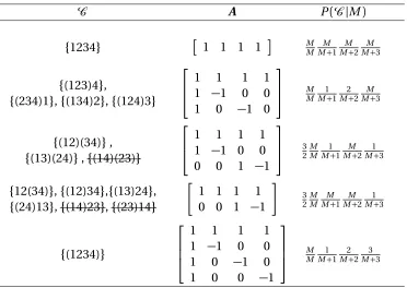
When splitting the parent into four children pixels, we use the one-step quad split-ting (White and Ghosal, 2011), rather than a two-step procedure (Kolaczyk, 1999a) of first vertical and then horizontal, because the former is rotationally invariant. We use the 4-person CRP model to specify the prior probabilities for quad splits, which corresponds to the tie ofξ’s. The configuration ofξ’s formed by subgrouping the four children is de-noted by_C, and let_Cbe the collection of all 15 possible configurations. These possibilities are given by a CRP with parameterM. For example, the configurationC = (123)4 means

ξ1=ξ2=ξ3, where the order of (1,2,3,4) is given below:

1 2 3 4

Given a smoothing parameterM in the CRP, the prior probability of each configuration P(_{C |}M)is given by a modified version of CRP(M), the CRP with parameterM. A possible modification is to remove 3 of the total 15 configurations:(14)23,(23)14 and(14)(23), which are only diagonally tied and unlikely to appear in a real image especially in the finest level of images. In this case, we scale the probabilities of other configurations of the same type to ensure that the total probability is 1. Table 2.1 displays the distribution under the modified CRP(M). The simulation results given later in Table 2.4 show that the removal of diagonal ties generally improves the accuracy slightly, but it can save substantial computation time, especially for 3D images (see Section 2.4) where computation is a major concern.

Conditionally on the grouping, a prior for ξ is given by a normal distribution. For notational convenience, we focus the discussion for one particular parent-child group. LetX = (X1,X2,X3,X4)be the observation of four children andX = X1+X2+X3+X4be

the observation corresponding to the parent. The prior distribution of the parameters

ξ= (ξ1,ξ2,ξ3,ξ4)is specified byN(0,τ2I). One natural constraint onξis that it should be summed to zero. Further, each configuration_C corresponds to some linear constraints for

(30)

Ta-ble 2.1 for all the constraint matrices associated with given configurations. By Lemma 2.4 presented in Section 2.6, the prior distribution ofξgiven each configuration_C which is equivalent to the conditionAξ=0, is given by:

ξ|C ∼N(0,(I −A0(A A0)−1A)τ2),

whereAis the constraint matrix corresponding to each configuration.

Table 2.1: Illustration of the corresponding constraint matrix A and prior probability P(_{C |}M)for given configuration_C. The column of_C contains all possible configurations belonging to the same tie structures, while the diagonally tied ones are crossed out. The constraint matrixAis for the first_C, while the other constraint matrices can be obtained by permuting the columns ofAaccording to the tieing structures. The last column is the prior probability P(C |M), which is shared by all configurations in the same category.

C A P(C |M)

{1234} 1 1 1 1 M_M _MM₊₁_MM₊₂_MM₊₃

{(123)4},

{(234)1},{(134)2},{(124)3} 



1 1 1 1

1 ₋1 0 0 1 0 ₋1 0



 M_M _M1₊₁_M2₊₂_MM₊₃

{(12)(34)},

{(13)(24)},{(14)(23)}





1 1 1 1

1 −1 0 0 0 0 1 ₋1



 3₂ M M

1

M+1

M M+2

1

M+3

{12(34)},{(12)34},{(13)24},

{(24)13},{(14)23},{(23)14}

1 1 1 1 0 0 1 ₋1

3 2 M M M M+1

M M+2

1

M+3

{(1234)}



 

1 1 1 1

1 ₋1 0 0 1 0 ₋1 0

1 0 0 −1

   M M 1

M+1 2

M+2 3

(31)

2.2.2 Posterior distributions

We shall derive the posterior distribution of_C given(M,τ)and the observationX assum-ing the model parameterσ2

0 =σ

2 _{is known. The estimation of the model parameter}_σ2 0

and smoothing parameters (M,τ) will be discussed in the Section 2.2.3. By the Bayes rule, we obtain the posterior probability of the configuration_C:

P(C |M,τ,X)∝P(C |M)P(X|C,τ,X),

whereX is the observation vector for the four children, andX is that of the parent, i.e.,X is the summation of all elements inX.

This is a discrete probability distribution with 12 distinct values, so they need to be scaled to sum to one. The first factor, P(_{C |}M), is given by the modified CRP. The second factor, P(X|C,τ,X)can be obtained fromξ_|C andX|ξby applying Lemma 2.5, presented in Section 2.6. From the discussion about the model assumptions and prior distributions, we have

X|ξ ∼ N(1

4X14+ξ,Σ1),

ξ|C ∼ N(0,Σ2), where

Σ1=σ2Σ0, Σ2=τ2(I −A0(A A0)−1A),

andΣ0=I−10₄(1410₄)−110₄; hereAis the constraint matrix corresponding to the

configura-tion_C. Applying Lemma 2.5, we can obtain

X|(C,τ,X)∼N(1

4X14,Σ1+Σ2). (2.6) The enforced constraintX1+X2+X3+X4=X makes the joint distribution rank deficient,

which can be reduced to a lower 3-dimensional multivariate normal by dropping one of the co-ordinates. We shall drop the last oneX4to make the covariance matrix nonsingular

in the computation. However, we shall keep all of them in the formulas to make them symmetric, and just remind the reader of the singularity issue when necessary.

(32)

distri-bution by conjugacy, namely,

ξ|C,X ∼N(Σ2(Σ1+Σ2)−1(X −

1

4X14),Σ2(Σ1+Σ2) −1_Σ₁₎

;

here the vectorξis summed to be 0, thus is lower dimensional as is the case in (2.6). Simi-larly we can drop the last oneξ4to address the singularity issue. The final estimate of each pixel in one parent-child group can be obtained by

b

ξ= X

C ∈C

P(C |M,τ,X)E(ξ|C,X) = X

C ∈C

P(C |M,τ,X)Σ2(Σ1+Σ2)−1(X −

1

4X14). (2.7) Similarly,

b

E(ξξ0_|_X_{) =} X

C ∈C

P(C |M,τ,X)[ξbbξ 0

+Σ2(Σ1+Σ2)−1Σ1].

Adding (2.7) across levels gives the estimate of the posterior mean of µj,k (see equa-tion (2.4) and (2.5)). Note thatξ’s over different levelsl are a priori independent and their likelihood factorizes, so they are a posteriori independent too. This allows to obtain the estimate of Var(µ2

j,k|X)by adding variances of the appropriateξvariables which add to

µj,k in view of their posterior independence.

2.2.3 Estimation of parameters

When the varianceσ2_{is known, we have two smoothing parameters:} _M _and_τ_{for each}

(33)

For each parent-child group, the marginal likelihood of the sample given (M,τ) and the group sum is

P(X|M,τ,X) = X C ∈C

P(_{C |}M)P(X|C,τ,X). (2.8)

Before maximizing (2.8), we pass to the logarithmic scale to make the algorithm more sta-ble. Since the optimization is conducted for the entire level, we need to formulate the target function pooling all the parent-child groups together. For levell = 1, 2, . . . ,L, the length of a row or column is 2l_{, and thus the number of such groups is 4}l−1_{. Using}_z _{as the}

index for the children groups, we can derive the target function as:

4l−1

X

z=1

log ¨

X

Cz∈C

P(_{C |}M)P(X_|C,τ,X) «

. (2.9)

The Newton-Raphson algorithm or grid search type algorithms can be applied with the decreasing constraint in(M,τ). We use a simplex search algorithm (Lagarias et al., 1998) which gives stable estimates. The selection of parameters is more critical for finer scales of the image. In practice, we use multiple starting points to ensure global maximization.

For real image data, the variance σ2 _{at each pixel is unknown. The parameter} _σ2

can also be estimated by maximizing the marginal likelihood similar to the estimation of

(M,τ). However, unlike(M,τ), which are estimated separately for each level of data,σ2

is fixed across different levels. Thus the optimization of the log-likelihood is much more computationally intensive, especially for images with large sizes. The method of moments estimation has a computational advantage and will be used here. For the(j,k)th children group in the(L−1)th level of the image, denote the indexes corresponding to the(j,k)th block as C(j,k) = {(j0_,_k0₎ _: _j0 ₌ ₂_j ₋_{1, 2}_j_,_k0 ₌ _2k₋_{1, 2k}_}_{. Let} _s2

j,k be the sample vari-ance for the dataXj0_,_k0, where(j0,k0)∈C(j,k), thens_j2_,_k is an unbiased estimate forσ2 if

µj0_,_k0(j0=2j−1, 2j;k0=2k−1, 2k)are all the same. Then an estimate ofσ2can be obtained

by averaging all the sample variances:

Ò

σ2₌ 1

4L−1 2L−1 X

j=1 2L−1 X

k=1

s_j2_,_k. (2.10)

Obviously, not all four children pixels have intensities coming from the Gaussian distribu-tion with the same means, such as if the children block contains a part of a boundary in the image. In that case,s2

(34)

the overall variation. But the effect will be not significant if the non-boundary pixels dom-inate the whole image, as showed by the following theorem. The proof of Theorem 2.2 is deferred to Section 2.6.

Theorem 2.2. Suppose that we observe an image X of size n = 2L _{in each direction. Let} the true image arise from the realization of a function g : (s,t) 7→µ(s,t) on the domain D= [0, 1]_×[0, 1]and be corrupted by independent Gaussian noise with mean0and variance

σ2_{at each pixel.}

Assume that the true surface g(·,·) is bounded by a constant m . Further assume that D =D1∪ · · · ∪ Dk,k <∞, whereDi0 =Di\∂Di is a convex set such that g(·,·)is Lipschitz continuous onD0

i,i =1, . . . ,k.ThenÒσ

2 _{defined in}_(2.10)_{is asymptotically unbiased and is}

consistent forσ2_{as n}_{→ ∞}_.

We can improve the finite sample performance of_Òσ2_{by the following modifications.}

Consider the sample variancess2

i,j,i,j =1, . . . , 2

L−1_{, as the new scalar responses, and}

de-note them as zt,t = 1, . . . , 4L−1. We know that the majority of zt have meanσ2 but the others have means larger thanσ2_{, for example the blocks containing boundaries.}

There-fore we could classify all s2

j,k’s into two groups via commonly used clustering methods such asK-means (Hartigan and Wong, 1979) withK =2. The two clusters are boundary-containing or boundary-free groups and we can use the mean ofs2

j,k’s in the boundary-free group to estimateσ2_{. As a more sophisticated alternative, a Gaussian mixture model can}

be used to classifyzt’s to the various groups:

zt =p1f1+p2f2+· · ·+pKfK

wherep1+· · ·+pK =1, andf1, . . . ,fK, are densities for normal distributions. An Expectation Maximization (EM) algorithm is used to estimate parameters (McLachlan and Peel, 2000) and has already been implemented in MATLAB. The number of componentsK can be se-lected by the Bayesian information criterion (BIC) using data. A simpler alternative could be to use just the fixed valueK =2, where the mean of the component with larger propor-tion is used as the estimate ofσ2_{. All the modifications improve the performance of}

Ò

σ2

(35)

2.2.4 Asymptotic properties

The proposed Bayesian denoising method enjoys some good convergence properties. Let

µ = (µj,k : j,k = 1, . . . , 2L)be the mean parameter of the image in the Bayesian model, andµ0 = (µ0_j_,_k : j,k =1, . . . , 2L)be the true value of the underlying mean of the observed image. Define a structure_Mby equality among neighboring values of the split parameters at any level. For example, the full model for the observed image is that the components of the underlying mean(µ_j_,_k : j,k =1, . . . , 2L₎_{are not at all tied among intensities. With} more specifications of ties, a structure becomes more restricted. Let the true structure be_M₀, and call any model that is broader than_M₀a compatible model; otherwise call it incompatible. A compatible model has fewer assumptions of ties than the true model, and thus will never contain any incorrect specification of ties but it may miss some correct ties. White and Ghosal (2011) showed that under the Poisson model for the image, as the total intensity tends to infinity, the posterior distribution of relative intensities is consistent and the posterior probability of the true model converges to one. A similar result holds in our setting of Gaussian noised images.

Theorem 2.3. For the Bayesian smoothing method with modified CRP, we have that (a) the posterior distribution ofµis consistent atµ0_as_σ_→_0;

(b) for any incompatible model M∗_{, the posterior model probability} _Π₍_M∗_|_X₎ _≤ exp(₋c/σ2₎_{for some constant c} _>₀_{almost surely for all sufficiently small}_σ_;

(c) for any compatible model M∗ _{that is different from the true model, the posterior} model probabilityΠ(M |X) = Op(σd), where d is a constant standing for the redundancy ofM∗_.

(36)

2.3 Simulation results for 2D images

In this section, we conduct a simulation study to judge the practical performance of the proposed Bayesian smoothing method using the Chinese restaurant process (Bayesian CRP). We compare with five other existing approaches, which are translation-invariant Haar (TI-Haar) estimation (Willett and Nowak, 2004), coarse-to-fine wedgelet (Castro et al., 2004), platelet (Willett and Nowak, 2003), nonparametric Bayesian dictionary learn-ing (BPFA) proposed by Zhou et al. (2012) and the conventional runnlearn-ing median method. All the implementations are completed in MATLAB.

The Gaussian model can be applied to a wide range of images, regardless of the quan-tity being measured for each pixel. They are much more applicable to the large photon images, or images based on a continuous quantity like intensity. The essential differences can be summarized according to the number of unique values of intensities in the image. Call them discrete images when there are a limited number of unique values and continu-ous when there are a large number of unique values. In our simulations, typical images from both discrete and continuous cases will be used. The image of the Shepp-Logan phantom (Jain, 1989) is discrete, while the Lena image is continuous. The Shepp-Logan phantom image contains ellipses with various absorption properties to mimic the outline of a head, which is widely used to test reconstruction algorithms. The Lena image is a real image typically used to measure the performance of smoothing algorithms. True intensity values in both images are within the range 0 to 1.

Cycle spinning is a common technique to remove visual artifacts in image reconstruc-tion (Coifman and Donoho, 1995; Willett and Nowak, 2004) and can be completed by aver-aging random or local shifts. We average 121 local shifts (11×11, which means a step size up to 5 in each possible direction) for the methods of Bayesian CRP, wedgelet, platelet and running median. The TI-Haar is translation invariant and hence it is not necessary to ap-ply local shifts any more, while the BPFA method already includes cycle spinning in terms of patches automatically. The tuning parameter for platelet is hard to specify. We use the value 0.1, which gives the smallest mean squared errors (MSE) for the Lena image when

σ=0.5. The length of the window for the running median method is fixed at 5. We esti-mateσ2_{by equation (2.10) with 2-means or Gaussian mixture models since the results are}

(37)

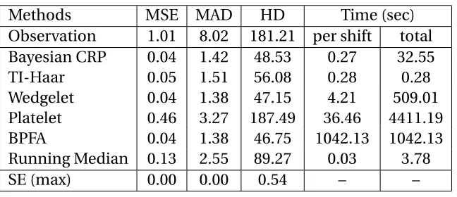
Table 2.2: Numerical comparison of smoothing methods for the phantom image when noise standard deviationσ=0.1. The mean MSE (_×10−2₎_{, MAD (}_×₁₀−2₎_{and HD (}_×₁₀−2₎

of 100 simulations are reported. The maximum standard error for each criterion is given by the last row. All methods except TI-Haar and Bayesian dictionary learning use 121 lo-cal shifts to remove artifacts. The running time for each lolo-cal shift and the total time are reported in the last two columns.

Methods MSE MAD HD Time (sec)

Observation 1.01 8.02 181.21 per shift total Bayesian CRP 0.04 1.42 48.53 0.27 32.55

TI-Haar 0.05 1.51 56.08 0.28 0.28

Wedgelet 0.04 1.38 47.15 4.21 509.01

Platelet 0.46 3.27 187.49 36.46 4411.19

BPFA 0.04 1.38 46.75 1042.13 1042.13

Running Median 0.13 2.55 89.27 0.03 3.78

SE (max) 0.00 0.00 0.54 – –

The performance of various methods are compared both visually and numerically. The visual performances to the two images are shown in Figure 2.1 and Figure 2.2 for obser-vations with light noise (σ=0.1). We can see that the smoothed images obtained by the proposed Bayesian approach are able to identify most of the features present in the true image. For example, the small ellipses are still visible after smoothing by the Bayesian CRP method, as well as Bayesian dictionary learning (BPFA) and running median. Both the Shepp-Logan phantom and Lena images show that TI-Haar, wedgelet and platelet tend to over-smooth, which miss features present in the true images. The platelet method de-pends on the selection of a tuning parameter, which may have caused its problematic per-formance. Figure 2.3 demonstrates the performance of all six methods for the Lena im-age with heavier noise (σ=0.6). We can see that the Bayesian CRP method reconstructs the key features such as the nose and the mouth, while achieving smoothing even though the observed image is heavily noised. TI-Haar and wedgelet tend to oversmooth and miss some features such as the boundary between the face and the arm. The platelet, BPFA and running median methods capture features but tend to overfit since the smoothed images are still grainy.

(38)

(a) Original (b) Observation (c) CRP (d) TI-Haar

(e) Wedgelet (f ) Platelet (g) BPFA (h) RM

(39)

Figure 2.2: Comparison of the Bayesian smoothing method with other approaches for the 512_×512 Lena image shown in (a). The noisy observation with standard deviationσ=0.1 is shown in (b). The six denoising methods (c)–(h) are respectively Bayesian CRP, TI-Haar, wedgelet, platelet, Bayesian dictionary learning and running median. All methods except TI-Haar and Bayesian dictionary learning use 121=11_×11 local shifts to remove artifacts.