Abstract: Future mobile communications involves high data rates across large coverage area, latency, reliability and large number of devices in small area. To achieve this, the systems are categorized based on their abilities and their potential at work such as higher Mobile Bandwidth, Ultra-Reliable Low Latency Communication systems employed with reduced latency. These connections require efficient resources based on time and frequency or Frequency-division duplexing (FDD) systems, and many antennas imply high pilot overhead. For eliminatory this problem, compressed sensing based channel estimation provides a suitable. Moreover, Bayesian method gives overtime in matter of estimation of channel performance for attaining desired achievable rates. The results of simulation have proved the effectiveness of proposed Bayesian compressed sensing based estimation of channel having minimum pilot overhead. Comparison of various techniques compressed with sensing based and traditional LS methods have been presented.
Index Terms: Bayesian Learning, Compressed sensing, Channel
estimation, Frequency Division Duplex, Gaussian Mixture, Massive MIMO.
I. INTRODUCTION
The huge demand of high data rates in 5G technology, the usage of conventional MIMO antenna system is needed to extend massive MIMO to increase the potential support of spectral efficiency, reliability & overall capacity in TDD/FDD cellular systems, detailed identification in [1]. The subsequent work analyzed on massive MIMO systems, more details in [2], to provide higher spectral efficiency, resultant using simple techniques of transmission and reception. Because of more number of transmitters and receivers are using at massive MIMO systems, the CSIT acquisition resembles as a most challenging problem detailed explanation in [18]. The base station receives pilot symbols from different antennas in the downlink channel, moreover to move backward to the BS with channel state information to analyze pre-coding coefficients. However, to calibrate for studying quantitatively the channel reciprocity for obtaining CSIT by training sequence in uplink having length independent of downlink antennas of transmission, many researchers presented that full duplex types is helped by time division duplexing (TDD) detailed research work in [4, 5]. Therefore,
Revised Manuscript Received on June 05, 2019.
T.Ravi Babu, Research Scholar, Department of ECE, GITAM Institute of Technology, (GIT) GITAM, Andhra Pradesh Visakhapatnam, India.
C.Dharmaraj, Professor, Department of ECE, GITAM Institute of Technology, (GIT) GITAM, Andhra Pradesh Visakhapatnam, India.
the precise accomplishment of CSIT at FDD massive MIMO systems over downlink training and the feed backed signal from the receiver is of great importance. However, as the work of calibration is relatively complex in TDD, the current cellular system prefers FDD for 5G systems.
In FDD systems no channel reciprocity attained due to usage different frequencies in uplink and downlink transmission. Usually, estimating pictures of the channel requires a specific sequence to train provided that information of the previous outputs received in course of training on standard procedure is available. Additional feedback is required for getting the statistics of non-stationary MIMO. To circumvent this situation, a novel technique of CSI determination along with feedback strategy giving accurate reliable CSIT having reduced complexity as well as overhead is desirable. Compressed sensing is offers suitable method for estimating short sequence type of sparse with unknown statistics identified in [11, 12, 23, 24]. In this paper, combined of LS and CS techniques are used to obtain estimation in FDD [15, 16, 24] having various of sparse and dense vectors. Due to improved recovery performance methods in [3, 17, 25], Bayesian estimation scores over other equivalent methods; it can increase monitoring of fractional space of the channel by reducing pilot overhead.
The remaining part of this paper is divided as per the following. Second Section discusses downlink and estimation models of noise. Third section discusses training sequence design and principle of estimation to existing technique, forth section discusses OMP and Bayesian approaches, fifth section practical issues and finally sixth section concludes.
II. SYSTEMMODEL Let 1, 2 M
h h C channel response between a Base station and two different user terminals. The fading model is given by
1 [(i1)L l ], l1, 2,3,...., ,L
h h (1)
Here h1andh2 represents the vectors of channel having
symbols respectively. These are orthogonal
1 2
[ H ] 0.
h h The separated signals x x1, 2transmitted by the
users, so that 1 1 1 1 1 2 2,
H H H
y x x
h h h h h due to the
orthogonality and non-zero vectors, the inter-user interference disappeared, so thath h1H 2 0.
The signal corresponds to nth symbol is
Performance Comparison of Downlink Channel
Estimation in FDD Massive MIMO using
CS-Aided and Bayesian Compressed Sensing
Methods for 5G Systems
[ ]
h [ ].x[ ]
H[ ]
y n
n
n
z n
(2) here h[ ] and x[ ]n n are the vectors for channel and the case corresponding to nth transmission symbol time with
2 2
x[ ] 1,
E n is gives SNR in presence of white noise. If
1 M
h C and 2 M
h C have independent random vectors with zero mean, such that
1 2 0 H
M
h h
(3)
This shows that the inner product between h1andh2.The multivariate circularly symmetric complex Gaussian distribution h h1, 2C,N ( ,0 IM), where IMis the MM
identity matrix [1, 2]. Hence, variance of the inner product (3) 1 /Mdecreases linearly with the number of antennas. The inner product ( 1H 2) / 0,
M
h h where as M ,does not
give that 1H 20
h h .The inner product h h1H 2 increases with M towards Rayleigh cases.
A. Downlink Channel estimation
Coherent transmission using CSIT is desirable. If the uplink feedback delay is neglected, data transmission is given by L T Pwhere L is coherence block of length L and Tp is channel training period. The block length is imperfect due to channel. The training time TP increases, while available channel are used for downlink transmission is decreases. Good channel training having small TP to desirable.
The received signal is given by
,
,
[ 1] 1 , [ 1] 2 ,..., [( 1) ]
T
i T p
H T
T i T i T
y i L y i L y y i L T
y
h X w
(4)
where x [1],..., x [ ] M Tp
T T T Tp
X C this is pilot sequence
having
tr(
X X
TH T)
T
p.B. LS Channel estimation
For LS channel coefficients are expressed as
, 1 ( ) LS T H
i i T T
T
h y X
(5)
Where 1
( )
H H
T
X X XX give inverse and pseudo-inverse ofXT, Tp Mrequiring large amount of downlink resources. The channel estimation can be done by short sequence. The length of the training sequence, Tp satisfying Tp k is sufficients ji( ). For training the k non- zero coefficients
constructed as k Tp T
X C and Mk matrix obtained from column vectors.
III. CS-BASEDCHANNELESTIMATION Simultaneous operation of LS and CS approaches is necessary for reducing training overhead. As the support of transformed channel vector changes sluggishly, this scheme can be based on two vectors considering previous support [6-9, 19].
A. Training Sequence Design
A fraction of total dimension k is use for determining the
values
1
,
s s
i T
i d IM i.The other part of length Tpk is
used to estimate
1
,
s c s
i T
i s IM i. The pilot is given by
, , ,
i T i d i s
X X X
(6) For estimating si d, the Xi d, can be given by
1
, i
i d d
X ψ X
(7) Here
X
d
C
k k is satisfies condition of orthogonalityX X
Hd d
I
k, with k can be obtained by LS filter. TheXi s, is used for the estimation of determinesi s, . Since,
si sis sparse. This can be calculated using CS method by this
condition 1
c
p i
T k .It can be restricted with a
compressed number.
1
, c ,
i H i s
X ψ Φ
(8) Here pertains to the estimate measured in CS method.
B. Principle of Estimation
At the receiver the value is determined by T, T, T, i T i d i s
y y y
where 1 , , , , , , h
s ( ) z
s z
i
T H T
i d T i i d i d
H T
T i M d i d
H T
T i d d i d
y
z
X I X X (9) and 1 , , , , , , hs ( ) z
s z
c i
T H T
i s T i i s i s
H H T
T i M i s
H H T T i s i s
y z
X I Φ Φ (10)
The matrix vector si d, is obtained fromy .i d, Under the LS
channel estimation approach, we can express the mean value of si d, gives ofsi d, in place ofy ,i s, the estimate of si s, comes
fromyi s, with condition of sparse algorithm.
IV. SPARCERECOVERYALGORITHMS
The CS channel strategy is employed by the OMP algorithm is presented in [8, 9, 13]. The OMP algorithm is one of the greedy methods, based on residual error and errors differences.
A. Orthogonal Matching Pursuit (OMP) Algorithm Starts with empty set of uncovered channel paths,
z
becomes measurement iteration is used.z
i i
h (11) Where hi is the sparse vector impulse of ith case. Fundamentally, two strategies are involved on the every iteration. Firstly, single delay of transmitting includes all the delays. This is sum of accumulated delay. Secondly to select as many uncovered paths is required to estimate gains. The OMP Algorithm procedure as follows:
1) Actuate the remaining error
0y
*i s, , with index0
and i = 1. 2) observe column
of the residual error i1.
3) i i1 { }ji is updated, where
1
arg max
{1, 2,...,
}
H
i j i
j
j
M
k
and j isth
j column
of matrix Φ.
4) Setting u ( ) ( )1 y*,
i i i i
H H
i M k i s
I Φ Φ Φ of
changing the residual error signal is estimated *
,
y
u .
i i s i
Φ
5) If iks, stop and evaluate ,
1 si s u .i
T
else, need
of continuation is there.
With the estimates si d, andsi s, , a primary estimate can be
obtained as
1
1 , ,
s ( ) s ( ) c s .
i i IM i d IM i s
(12) When OMP is used for process of getting better, due to noise, closing of rule 5 covers residual error. So, if
2
,
s i
i
k or
stop is applied η is threshold depending onnoise. In proposed scheme the iteration extends up toiks. The support can be chopped after results are considered. For the CS channel estimation [20-22], the pilot is designed when
i
S is sparse (kM)
H CS CS
X ΨΦ (13) HereΦCSis a compressive measurement matrix. At this stage combination of the techniques mentioned in [15, 16] is necessary.
However, the OMP solves the optimization problem:
0
min ,
i i
h h such that
y
i
Φh
i 2
OMP . TheparameterOMPis dependent on hiand variance. Compared to LS on OMP, the BCS Algorithm does not need a prior knowledge statistics.
B. Bayesian Compressed Sensing (BCS) Algorithm Bayesian channel estimation approach improves effectively by allocating the same pilots to spatially separating users in different cells. Acquiring to the culmination it requires some overhead of estimating the covariance matrices and computation complexity.
The distribution ofhishould be known. For this the following two conditions are, the important. Firstly, it each element of
i
h consists of few random variable elements of hi need substantially distant variances, more specifically, some instances are very small however a few are large. After the observations, the elements are modeled as hi [hi k, ] Gaussian-mixture (GM) distribution is being a mean.
2 2
, , , ,
1
( ; , ) ( ;0, ),
L
i k n i i l i k i l l
P
h
N
h(14)
Where
N C
(
h
i k,;0,
i l2,)
is the PDF and gives mixingprobability [3]. The parameter
i2,1.is minimized. The rest ofthe GM components
2
,, , 2L i l i l l
give a part of greater
values. Variance is decided by L gives the number of different variances inhi. Finally, it is assumed that the BK-dimensional (BK=T) higives this
, 1
( ; ) ( ; ),
BK
i i i k i k
P
P
h h
(15)
For omitting i from P( ;hii) and index i
from
i l,,
i l2,,
i,
i,
i. The parameters
2
,, , 1 L i l i l l
are a
learning algorithm. There are 2 algorithms (i) AMP algorithm is presented in [8, 9] (ii) Bayesian algorithm is presented in [5,
14, 25].The elements of hifollow the Gaussian Mixture
pattern for earlier values ofi. To obtain the most profitable
values of i,hi k, is termed as a output of AMP. From Bayes
theorem, the hi k, is calculated from the output as
, ,
, , , ,
, , , , ,
( )ˆ ( AMP)
( ; ; ) ( ; )
( ; ; ) ( ; )
AMP i k i k
i k i k i k i k i i k i k i k i k i i k
h P h
h a v P h
h a v P h dh
N N C C (16)
For ai k, and vi k, change with iteration i
with
AMP(hi k, )plugging the GM prior (15) into (16) then weget
, , , , , , , , 1
( ) ( ; ; )
L
AMP i k i k l i k i k l i k l l
h Q h
N
C(17)
Where
2
, , , ,
, , 2
1 , , , ,
( , )
,
( , )
i l i k i l i k i k l L
l i l i k i l i k
a v Q a v N N C C (18a) 2 ,
, , 2 ,
, ,
, i l i k l i k
i l i k
a v
(18b)
2 , , , , 2
, ,
. i l i k i k l
i l i k
v v
(18c)
In [10] using EM technique and Bayesian Channel estimation [25] a proper expression can be made for
estimation of H.
Algorithm 1 BCS-Based Algorithm
For Φ based inputs and Observation matrix y.
1: The first formulationsLandˆ10are selected: 2. Fori1to N do
3: t1; 4. Repeat
5: AMP Algorithm:
Generate ( t, ) ( t, ; t, ; t, ) i k i k i k i k
Q h
N
h a v with ˆt 1 i fromAMP Algorithm; 6: Parameter learning: 7: Learn the noise Variance; 8: Update the GM priors ˆ ;it 9: t t 1;
10: Until 12
, , t t k ai k ai k
;
11: Compute 0 0 1 1
ˆ ˆ
( , ) ( ,t t)
i i i i
Outputs: Return the Estimated Channel H.
The Steps 7–8 are used for earlier values including noise for obtaining convergence. In Step 11, the learned parameter of estimatinghiis used with the
estimation performance additionally improves convergence.
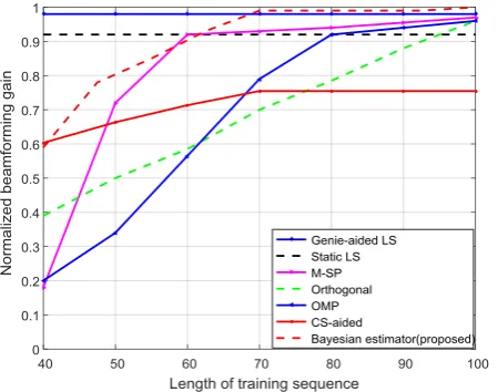
[image:4.595.310.536.222.403.2]V. DISCUSSIONSANDSIMULATIONRESULTS The performance of Bayesian Gaussian mixture needs to be compared with other estimation schemes. OMP is used as sparse recovery algorithms,. The baseline schemes can be summed up as Genie-aided LS: For this, value of i is considered in subspace. LS estimate is then carried out. For Static LS, the value of first block is considered. In Random LS, orthonormal sequence is used for trained LS. In OMP, random Gaussian matrix M T Pis selected. M-SP algorithm gets back the channel initiated with the previous information, similar to CS-aided scheme.
Fig.1.Normalized gain vs training sequence with SNR = 20 dB.
The Fig 1 illustrates beam forming for gain various schemes in which training is done at T 20dB, (k to M). It
cannot be utilized by random orthogonal pilot. OMP plus CS based estimator’s fails because of reduced additional parameters. It can be inferred that sparsity cannot be determined by Compressing Sensing.
Fig.2.Normalized mean square errors the mismatched parameter with SNR = 20 dB.
Moreover, as support where is sluggishly so that a static method can give wrong results compared with random variables best methods. Because the coefficients for ksan estimate of supporting parameters cannot be done by static
methods, M-SP is better than traditional OMP. Basically construction can estimate sparse vector which is similar to the inverted value of the earlier structure by including shorter program for training.
Fig 2 displays the degradation of performance of estimation schemes such as M-SP and CS-aided with prior support information with parameter mismatch. The gradation of CS-aided is low whereas M-SP is likely to have more mismatched. Bayesian CS-aided channel estimation outscores the CS-aided and is of their order of generalized scheme. The results show the efficacies of separation are clear from the results shown.
[image:4.595.56.281.227.404.2].
Fig.3.NMSE vs SNR of estimation schemes with M=100 and k=40
Fig. 3 illustrates NMSE - SNR for the case of changing SNR. It is formed that CS algorithms is basically noise sensitive. All the estimation schemes connected to CS shows poor result in low SNR portion. In comparison to this, LS based schemes have less error. For SNR15dBis, Bayesian scheme is better than Static LS and as reasonably good performance. Overall, the performed Bayesian method has less error than conventional CS techniques.
VI. CONCLUSION
REFERENCES
1. E. G. Larsson, F. Tufvesson, O. Edfors, and T. L. Marzetta, “Massive
MIMO for next generation wireless systems,” IEEE Commun. Mag.,
vol. 52, no. 2, pp. 186–195, Feb. 2014.
2. TV. Chen, E. Bjornson “Massive MIMO Communications” pp. 77-116, Springer, 2017
3. X Cheng, M Wang, Y Guan, Ultra wideband channel estimation: a Bayesian compressive sensing strategy based on statistical sparsity. IEEE Trans. Vehicular Technol. 64(5), 1819–1832 (2015).
4. Y. Shi, J. Zhang, and K. B. Letaief, “CSI overhead reduction with stochastic beam-forming for cloud radio access networks,” in Proc. IEEE Int. Conf. Communications (ICC), Sydney, Australia, Jun. 2014,pp. 5154–5159.
5. S Ji, Y Xue, L Carin, Bayesian compressive sensing. IEEE Trans. Signal Process.56(6), 2346–2356 (2008).
6. S. Nguyen and A. Ghrayeb, “Compressive sensing-based channel estimation for massive multiuser MIMO systems,” in Proc. IEEE
7. X. Gao, F. Tufvesson, and O. Edfors, “Massive MIMO channels -measurements and models,” in The 47th Annual Asilomar Conf. Signals, Systems, and Computers, Pacific Grove, California, U.S.A., 2013.
8. D. L. Donoho, A. Maleki, and A. Montanari, “Message passing algorithms for compressed sensing,” Proc. Nat. Acad. Sci., vol. 106, no. 45, pp. 18 914–18 919, 2009.
9. S. Rangan, “Generalized approximate message passing for estimation with random linear mixing,” in Proc. IEEE Int. Symp. Information Theory (ISIT), Saint Petersburg, Russia, Aug. 2011, pp. 2168–2172. 10. J. P. Vila and P. Schniter, “Expectation-maximization
Gaussian-mixture approximate message passing,” IEEE Trans. Sig. Process., vol. 61, no. 19, pp. 4658–4672, Oct. 2013.
11. W. U. Bajwa, J. Haupt, A. M. Sayeed, and R. Nowak, “Compressed channel sensing: A new approach to estimating sparse multipath channels,” Proc. IEEE, vol. 98, no. 6, pp. 1058–1076, Jun. 2010. 12. P. H. Kuo, H. T. Kung, and P. Ting, “Compressive sensing based
channel feedback protocols for spatially-correlated massive antenna arrays,” in Proc. IEEE Wireless Communications and Networking Conf. (WCNC 2012), Paris, France, Apr. 2012.
13. Y. C. Pati, R. Rezaiifar, and P. S. Krishnaprasad, “Orthogonal matching pursuit: Recursive function approximation with applications to wavelet decomposition,” in Proc. 27th Annu. Asilomar Conf. Signals, Systems, and Computers, 1993, pp. 40–44.
14. S. Ji, Y. Xue, and L. Carin, “Bayesian compressive sensing,” IEEE Trans.Sig.Process., vol. 56, no. 6, pp. 2346–2356, Jun. 2008. 15. N. Vaswani, “LS-CS-residual (LS-CS): Compressive sensing on least
squares residual,” IEEE Trans. Signal Process., vol. 58, no. 8, pp. 4108- 4120, Aug. 2010.
16. N. Vaswani, “LS-CS-residual (LS-CS): Compressive sensing on least squares residual,” IEEE Trans. Signal Process., vol. 58, no. 8, pp. 4108- 4120, Aug. 2010.
17. M Carlin, P Rocca, G Oliveri, F Viani, A Massa, Directions-of-arrival estimation through Bayesian compressive sensing strategies. IEEE Trans.AntennasPropagat.61(7), 3828–3838 (2013).
18. J. Shen, J. Zhang, E. Alsusa, and B. Letaief, “Compressed CSI acquisition in FDD massive MIMO: How much training is needed?”
IEEE Trans. Wireless Commun., vol. 15, no. 6, pp. 4145-4156, Jun. 2016.
19. X. Rao and V. K. N. Lau, “Compressive sensing with prior support quality information and application to massive MIMO channel estimation with temporal correlation,” IEEE Trans. Signal Process., vol. 63, no. 18, pp. 4914-4924, Sep. 2015.
20. T.Ravibabu and et.al “Performance Analysis of Sparse MIMO-OFDM Channel Estimation Using Spatial and Temporal Correlations” International Journal of Science and Research 5 (01), 942-945. 21. T. Ravibabu and C.Dharma Raj, “BER Analysis of spatial
multiplexing and STBC MIMO-OFDM System”2018 4th IEEE International Conference on Devices, Circuits and Systems (ICDCS),pp- 110-116, Mar 2018
22. Y.Han, J. Lee and David J.Love, “Compressed Sensing-Aided Downlink Channel Training for FDD Massive MIMO Systems” IEEE Trans. On Communications., vol. 75, issue 7, pp. 2852-2862, july. 2017.
23. Adinarayana.V, K. Murali Krishna, P. Rajesh Kumar. K.Lakshmi Narayana “Performance Comparison of Compressive Sparse Channel Estimation and feedback in 5G for hyper MIMO system” IEEE conference ICCS, Dec 2017.
24. N.Vaswani, “LS-CS-residual (LS-CS): Compressive sensing on least squares residual,” IEEE Trans. Signal Process. vol. 58, no. 8, pp. 4108- 4120, Aug. 2010.
25. CK. Wen, S. Jin, KK. Wong, JC. Chen and P.Ting“ Channel estimation for massive MIMO using Gaussian Mixture Bayesian Learning” IEEE Trans. On wireless Communications., vol. 14, issue 3, pp. 1356-1368, Oct. 2014.
AUTHORS PROFILE
T. Ravi Babu received his B.Tech and M.Tech degrees in Electronics and Communication Engineering from JNTU University, Kakinada, India, in 2005 and 2010 respectively. He is an Research scholar in GITAM Institute of Technology (GIT), GITAM, Visakhapatnam. His area of research includes Channel estimation on 4G/5G wireless communications, MIMO-OFDM, Massive MIMO, fading Channels. He has 10 years teaching 7 years Industrial experience. He has supervised and guided various projects for UG and PG level. He is a Member of Indian Society for Technical Education (MISTE).