Development of a software for simulating active force control schemes of a two-link planar manipulator

Jurnal Teknologi, 43(A) Dis. 2005: 49–72 © Universiti Teknologi Malaysia

DEVELOPMENT OF A SOFTWARE FOR SIMULATING ACTIVE FORCE CONTROL SCHEMES OF A TWO-LINK PLANAR

MANIPULATOR

MUSA MAILAH1* & POH YANG LIANG2

Abstract. The paper describes the development of a software in the form of an interactive computer program that integrates a number of robotic control schemes with the active force control (AFC) strategy as the key element of the robotic system that assumes a rigid two-link planar configuration. The various AFC schemes are employed in conjunction with a number of conventional and intelligent techniques embedded in the main control loop to approximate the estimated inertia matrix of the robot arm. The schemes have been individually developed and rigorously experimented through simulation studies. The results of these studies clearly indicate that the AFC technique provides a practical solution to enhance the robustness of the robotic system even in the wake of uncertainties, disturbances and varied loading conditions. Thus, it is deemed useful to develop software that can integrate a number of individual AFC schemes into a single program using a graphic user interface (GUI) technique. In this manner, the user can effectively select and execute any scheme by the manipulation of a few keystrokes or buttons of the input devices. This resulted in a program that is user friendly, readily accessible, flexible and proved very convenient. On top of that, the graphical results can be observed and analysed on-line while the program is running. By using MATLAB and its GUI facility, all the AFC schemes already described in the previous works such as the AFC with crude approximation method, AFC and Iterative Learning (AFCAIL), AFC and Neural Network (AFCANN), AFC and Fuzzy Logic (AFCAFL), and AFC and Genetic Algorithm (AFCAGA) schemes were linked into a single menu-driven program where each of the scheme can be easily selected and executed by the user. A classic proportional-derivative (PD) control scheme was also included in the program for the purpose of benchmarking.

Keywords: Active force control, robot arm, estimated inertia matrix, graphic user interface

Abstrak. Kajian ini adalah berkaitan dengan pembangunan perisian dalam bentuk suatu aturcara komputer berinteraktif yang menyepadukan beberapa skema kawalan robotik dengan kawalan daya aktif (AFC) sebagai elemen utama melibatkan tatarajah sebuah lengan robot planar tegar dua-sendi. Skema AFC yang digunakan bersama dengan beberapa kaedah konvensyenal dan pintar dimuatkan ke dalam gelung kawalan utama untuk mendapatkan matriks inersia anggaran lengan robot. Skema robot telah dibangunkan secara individu menerusi kajian yang dilakukan sebelum ini. Hasil daripada kajian yang telah dijalankan menunjukkan bahawa teknik AFC menyediakan suatu penyelesaian praktik untuk menambahkan lagi kelasakan sistem walaupun disertai dengan pelbagai keadaan tidak menentu, gangguan dan bebanan. Oleh yang demikian, adalah dirasakan perlu untuk membangunkan suatu perisian yang dapat menyepadukan kesemua skema AFC tadi menjadi satu program menerusi penggunaan kaedah antara muka grafik pengguna 1&2

Department of Applied Mechanics, Faculty of Mechanical Engineering, Universiti Teknologi Malaysia, 81310 Skudai, Johor Bahru.

(GUI). Dengan itu, pengguna boleh memilih dan menjalankan kerja simulasi skema yang dipilih dengan mudah melalui operasi menekan papan kunci atau butang pada alat masukan. Ini menghasilkan suatu aturcara yang berbentuk mesra pengguna, mudah dicapai, bolehsuai dan terbukti keberkesanannya. Selain daripada itu, hasil keputusan secara grafik dapat ditunjukkan serta dibuat analisis secara dalam-talian semasa aturcara sedang berjalan. Dengan menggunakan MATLAB dan kemudahan GUInya, kesemua skema AFC yang telah dikaji sebelum ini seperti AFC menggunakan kaedah anggaran kasar, AFC bersama kaedah pembelajaran berlelaran (AFCAIL), AFC bersama rangkaian neural (AFCANN), AFC bersama logik kabur (AFCAFL), dan AFC bersama algoritma genetik (AFCAGA) dapat dihubungkan ke dalam satu aturcara berasaskan menu di mana setiap skema boleh dipilih dan dijalankan oleh pengguna. Suatu skema kawalan berkadaran campur terbitan (PD) juga dimuatkan ke dalam aturcara sebagai kayu pengukur terhadap keberkesanan skema AFC.

Kata kunci: Kawalan daya aktif, lengan robot, matriks inersia anggaran, antara muka grafik pengguna

1.0 INTRODUCTION

Control of a robot arm has been a subject of active research for the last two decades. A number of control methods have been proposed to achieve stable and robust performance ranging from a simple classical proportional-derivative (PD) control to the more advance methods such as adaptive and intelligent control. The PD control is quite efficient and stable at low speed operation and with minor disturbances [1]. However, in view of the current robotic applications that are becoming more complex and challenging, there is a need for a more robust and effective control method. One of such method is the active force control (AFC) strategy that had been introduced in the early eighties [2]. This method has demonstrated very robust performance of the dynamic systems in the presence of disturbances, uncertainties and changes in the system’s parameters [3, 4]. Throughout the years, a number of research works have been carried out to further investigate the capabilities of the method including the incorporation of various intelligent mechanisms to effect the control action.

2.0 PROBLEM STATEMENT AND STUDY APPROACH

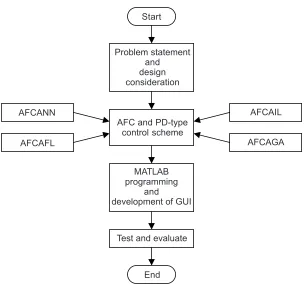
to accomplish the task of developing the desired program that shall fulfil all the requirements mentioned earlier. Figure 1 shows the approach that is used in the study.

Before discussing the details regarding the software development, it is useful to highlight the basic theories and underlying concepts associated with the relevant components of the control schemes considered in the study.

3.0 DYNAMIC MODEL OF THE ARM

The dynamic model of the arm can be described as follows [1]:

( )

( )

q d

T =H θ θ+h θ θ, +T (1) where

T_q : vector of actuated torque at joint H

HH

HH : N × N dimensional manipulator and actuator inertia matrix

and

,

θ θ θ : vectors of joint position, velocity and acceleration respectively h : vector of the Coriolis and centrifugal torque

T_d : vector of the external disturbance torque

Start

Problem statement and design consideration

AFC and PD-type control scheme

MATLAB programming

and development of GUI AFCANN

AFCAFL

AFCAIL

AFCAGA

Test and evaluate

End

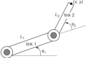
The gravitational term is not considered since the arm is assumed to move in a horizontal plane. In the study, a rigid two-link planar manipulator is used as shown in Figure 2.

4.0 ROBOT CONTROL

It is the ultimate aim of any robot control to ensure that the performance of the system is in line with the desired command. In this case, the robot is instructed to track specified trajectories accurately and robustly in the presence of disturbances. Two types of feedback control methods relevant to the study, namely the PD control and AFC shall be briefly described in the following sections.

4.1 Classical PD Control

The basic PD control algorithm of a robot system that described the actuated torque at a joint is [1]:

q p d

T =K e K e+ (2)

or Tq =Kp

(

)

(

)

where

K_p and K_d : proportional and derivative gains respectively

and

e e : joint position error and its derivative respectively

and _d

θ θ : desired joint position and velocity respectively and d

θ θ : actual joint position and velocity respectively

A block digram of the PD control scheme applied to a robotic system is shown in Figure 3.

Figure 2 A representation of a two-link planar manipulator link 1

L₁

L₂

(x, y)

θ2

θ1

4.2 Active Force Control

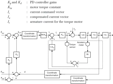
Active Force Control (AFC) is a very robust control scheme first proposed by Hewit and Burdess [3]. It is based on the well-known principle of invariance which relies on estimated and measured values of the relevant parameters that can render a dynamical system stable even in the presence of disturbances and uncertainties. The schematic of such a scheme applied to robot control can be seen in Figure 4. The notation used in Figure 4 is as follows:

K_pand K_d : PD controller gains K_tn : motor torque constant I_c : current command vector I_a : compensated current vector

I_t : armature current for the torque motor

Figure 3 A PD robot control scheme Desired

trajectory

Position sensor

PD controller Actuator Robot arm

Actual trajectory

Figure 4 AFC scheme applied to a robot arm + _ + + ++ + + _ _ + _ + + + + Coordinate

transformation IN/Ktn

Coordinate transformation Coordinate transformation Torque sensor Accelero-meter Ktn 1/Ktn Kd Kp Td Tq It Ic

1/H 1/s 1/s

IN

Td*

H : modelled inertia matrix of the robot arm

IN : estimated inertia matrix of the robot arm T_d* : estimated disturbance torque

T_q : applied torque

x and x_bar : vectors of the actual and desired positions respectively in Cartesian space

and

ref xref

θ : reference acceleration vectors in joint and Cartesian space respectively

In AFC, the important equation is as follows:

*

d q

T =T −INθ (4)

The expression can be simplified as:

*

d tn t

T =K I −INθ (5)

where

q tn t

T =K I (6)

The main computational burden in AFC is the product of the estimated inertia matrix (IN) with the angular acceleration of the arm before being fed into the AFC feed forward loop. Apart from that, the output of the system (in Cartesian space) needs to be computed from the joint angle space via forward kinematics operation. A controller in the outer loop should be added to the AFC component, thereby establishing an effective two degrees-of-freedom (DOF) controller. Normally, a classic PD control in the outer loop would suffice. However, in the study, a modified PD scheme is proposed here. It is known as resolved motion acceleration control (RMAC) which could improve the overall performance of the control system by providing a reference acceleration command [6]. RMAC is governed by the following equation:

(

)

(

)

ref bar p bar d bar

x =x +K x − +x K x −x

₍₇₎

Knowing that the performance of the AFC depends largely on appropriate value of IN, the method to estimate this inertial parameter is of considerable importance. Both conventional and intelligent methods of estimating IN are employed in the study. The former utilises a heuristic approach by simply assuming suitable IN

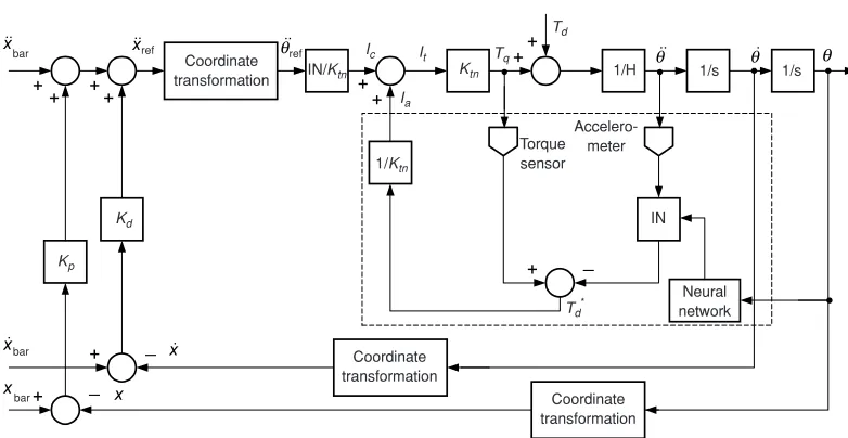
4.3 Active Force Control and Neural Network (AFCANN)

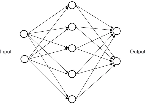
Neural network as an artificial intelligence (AI) technique has been known to have capability in approximating any arbitrary non-linear function to an acceptable degree of accuracy [13]. Generally, the basic structure of the network consists of a series of three layers that correspond to the input-hidden-output layers. Each layer possesses a number of neurons which are interlinked and interconnected with biases and weights assigned. Together, they form parallel processing units. Network with biases, a sigmoid layer and a linear output layer is capable of approximating any function with finite number of discontinuities. It is either trained through supervised or unsupervised learning procedure.

In the study, a multilayer feed-forward neural network with an error back propagation (BP) algorithm (a type of supervised learning method) was used to estimate the IN. The structure assumes a 2-5-2 configuration which corresponds to the number of neurons (nodes) in the input-hidden-output layers respectively [6]. The input variables are the joint positions, θ of the robot arm while the output is the computed IN. The implementation of the neural network was accomplished in two phases, namely the off-line training and the on-line implementation. The network was first trained off-line using a set of training data comprising 300 input-output pair prior to the on-line implementation of the neural network in the AFC scheme. The trained network resulted in the computation of fixed network weights and biases that are needed for the on-line phase. Figure 5 shows the neural network architecture used in the study.

The BP learning rule was used to adjust the weight and biases of the networks in order to minimize the sum-squared error (SSE) of the network. This is accomplished

Figure 5 A multi layer feed forward neural network with a 2-5-2 configuration

by continually changing the value of the network weights and biases in the direction of the descent with respect to error.

SSE can be expressed as

(

)

d

SSE=

∑

where

y_d : desired output vectors y : actual output vector

The weight adaptation mechanism with momentum factor and learning rate in the BP algorithm can be mathematically described as follows [14]:

( )

( ) (

)

_{( )}

W i , j m W i , j m l d i p j

∆ = ∆ + − (9)

where

∆W : weight change matrix l_r : learning rate

m_c : momentum constant

d : delta vector (derivatives of error vector) p : current input vector

BP algorithm, sometimes known as the gradient descent method with momentum, consists of changing or adjusting each weight connection proportionally to the generated error in the direction that decreases the error as rapidly as possible. The amount of adjustment is governed by two control parameters: the learning rate and momentum constant. The fully trained neural network can be treated as a black box for the on-line implementation and computation of the ‘optimised’ IN. The box is directly embedded into the AFC scheme to estimate IN during the actual operation of the robot arm. The incorporation of the neural network mechanism in the AFCANN scheme is shown schematically in Figure 6.

4.4 Active Force Control and Fuzzy Logic (AFCAFL)

Fuzzy logic is a superset of conventional (Boolean) logic that has been extended to handle the concept of partial truth-truth values between ‘completely true’ and ‘completely false’. The basic fuzzy logic concept is as shown in Figure 7.

or Boolean rules) to determined the dynamics of the controller as a response to the given fuzzy inputs. It is then passed through a defuzzification process using an averaging technique to produce crisp output values. The centroidal or centre of gravity method is described by the following equation:

( ) ( ) X X x .xdx x x dx µ = µ

∫

∫

The method is graphically depicted in Figure 8.

Figure 7 Fuzzy concept Crisp input

Fuzzification

Rules evaluation

Defuzzification

Crisp output

Figure 6 The AFCANN control scheme

+ + ++ + + _ _ + _ + + + + Coordinate

transformation IN/Ktn

Coordinate transformation Coordinate transformation Torque sensor Accelero-meter Ktn 1/Ktn Kd Kp Td Tq It Ic

1/H 1/s 1/s

IN

Td*

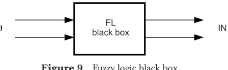
The completely designed fuzzy logic component can then be treated like a black box as shown in Figure 9. Note that the input of the black box is the vector of joint positions and the output being the inertia matrix.

Once the FL black box is appropriately designed, it can be directly embedded into the AFC loop to estimate INININININ as depicted in Figure 10.

Figure 8 Centroidal method

µµµµµX

x–

x

Figure 9 Fuzzy logic black box FL

black box IN

θ

Figure 10 AFCAFL control scheme

+ + ++

+

+ _ _

+ _ +

+

+ +

Coordinate

transformation IN/Ktn

Coordinate transformation

Coordinate transformation Torque sensor

Accelero-meter Ktn

1/Ktn

Kd

Kp

Td

Tq

It

Ic

1/H 1/s 1/s

IN

Td*

Ia ref

bar

bar bar

Fuzzy logic

ref

θ

4.5 Active Force Control and Genetic Algorithm (AFCAGA)

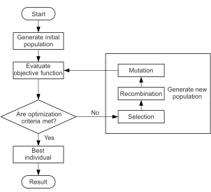
Genetic algorithm (GA) search method is based in the mechanism of evolution and natural genetics. GAs generate a sequence of population using selection and search mechanisms involving the process of crossover and mutation. GA operates on a population of potential solutions applying the principle of survival of the fittest to produce better and better approximations to a solution. At each generation, a new set of approximations is created by process of selecting individuals according to their level of fitness in the problem domain and breeding them together using operators borrowed from natural genetics. This process leads to the evolutions of populations of individuals that are better suited to the current environment then the individual that were created from, just as in natural adaptation.

Figure 11 shows a flow chart on how this algorithm works. To use a GA, a solution must be presented to the problem as a genome (or chromosome). The genetic algorithm then creates a population of solutions and applies genetic operators such as mutation and crossover to evolve the solutions in order to find the best one(s). In this case, track error will be feed into the algorithm to search for a better IN for the AFC schemes as shown in Figure 12.

In GA, fitness function has been chosen to evaluate the objective function using equation.

Figure 11 Structure of a single population evolutionary algorithm Start

Generate initial population

Evaluate objective function

Are optimization criteria met?

No

Mutation

Best individual

Result Yes

Recombination

Selection

Fitness function, 1 1 f E = + (11) where, ( ) 0 t t

E e t

= =

∑

E : sum of the track error from rest to the completion of a full circular trajectory

Figure 13 shows the proposed AFCAGA control scheme and the way GA component is embedded into the control strategy as the IN estimator.

Figure 12 GA for optimizing INININININ

GA IN

e

AFC

Figure 13 AFCAGA control scheme

+ + ++ + + _ _ + _ + + + + Coordinate

transformation IN/Ktn

Coordinate transformation Coordinate transformation Torque sensor Accelero-meter Ktn 1/Ktn Kd Kp Td Tq It Ic

1/H 1/s 1/s

IN

Td*

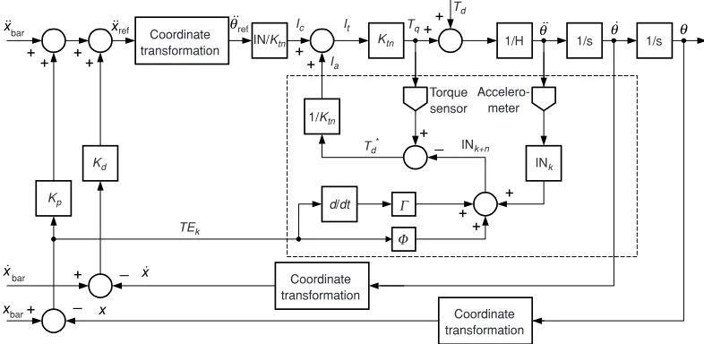
4.6 Active Force Control and Iterative Learning (AFCAIL)

From the word ‘iterative’, it is understood that the work is done again and again, over and over again. Through the iteration process, the intelligent will improve itself and reduce the error. Arimoto and co-workers are the first to propose iterative learning method to robot control. As the number of iteration, k(t) increases, k→∞, for t∈[0,tstop], the track error, e converge to zero. One of the learning algorithms proposed by Arimoto et al. is as follows [6]:

1

k k k

d

y y e

dt

+ = +_φ + Γ _ (12)

where,

y_k+1 : next step value of the output y_k : current output value

e_k : current positional error input given by e_k = x_d – x_k φ and Γ : suitable constants or learning parameters.

This expression can be simply called the proportional-derivative or PD type learning algorithm. In AFC, the above algorithm can be slightly change to suit the application and is given as follows:

1

k k k

d TE dt + = +_ + Γ _

IN IN φ ₍₁₃₎

where,

IN_k+1 : next step value of the output

IN_k : current output value

TE_k : current positional error input given by TE_k = Σ

(

)

The implementation of AFCAIL to a robot arm is shown in Figure 14. The box (shown in dashed lines) represents the most important part of the proposed scheme, which integrates AFC and the learning algorithm.

5.0 DESIGN CONSIDERATION IN SOFTWARE DEVELOPMENT

+ + ++ + + _ _ + + + + + +_{_} + +

(1) Software features

The software should be PC Window-based and designed in such a manner that it exhibits a user-friendly and interactive environment accomplished through the use of a GUI technique. It should also feature easy-to-use menu driven facility (with push-button feature) and sufficient on-line assistance with appropriate error messages prompting. The clicking operation of the pointing device, i.e. mouse to execute the selected control scheme should be minimal. The graphics should be simple, clear and appealing. The software should also offer adequate flexibility in dealing with changes to the system synonymous to an open-architecture design. In other words, the user can customize part of the system to include desired functions and additional features. On top of that, the graphical simulation results should be made available on-line through the computer screen for instant observation and analysis.

(2) AFC schemes

There are various AFC schemes involved, namely the ‘pure’ AFC, AFCANN, AFCAFL, AFCAGA and AFCAIL. The schemes were largely based on the method that is used to estimate the inertia matrix of the robot arm. Thus, the design of the program should take into account the capability of the program to provide users to readily select the scheme/s he wish to apply in simulating the desired robot control. In addition to that, a PD-type control scheme is also deliberately included due to the fact that it (or its variant) is coupled with all the AFC schemes. Pure PD control scheme is incorporated into the program for the purpose of benchmarking.

Figure 14 AFCAIL control scheme

Coordinate

transformation IN/Ktn

Coordinate transformation Coordinate transformation Torque sensor Accelero-meter Ktn 1/Ktn Kd Kp Td Tq It Ic

1/H 1/s 1/s

INk

Td*

(3) Operating conditions

In this part of the program, the user shall state the desired operating conditions. These include parameters such as the robot’s end-point velocity, simulation parameters (starting and stopping times, step size and integral algorithm), controller gains, initial conditions and parameters related to the respective intelligent mechanisms (learning parameters, momentum constant, error goals etc.). The design should also consider appropriate default values for all the parameters to assist new users in particular.

(4) Loading conditions

The loading conditions relate to the manipulation of specific forces/torques that are prevalent (either deliberate or otherwise) in the robot system. These include all forms of external disturbances and payload mass at the robot’s end-effector. In the developed program, it is expected that the user will define the specific type of disturbances acting on the robot arm. In the study, constant applied force, linear spring force, harmonic force, pulsating force and the hybrids (combination) were modelled and can be readily selected for the simulation work. It should also be noted that all motors employ direct drive transmission and hence no gear ratios were ever considered. In addition, the friction effects were not explicitly modelled in the study. In any case, it is expected that the AFC scheme should be able to counteract most of the inherent or applied disturbances including friction. However, future works could include this model and others.

5.1 Parameters Handling

A number of parameters related to the execution of the control schemes have to be clearly identified before the simulation study. These are the simulation parameters, robot physical parameters, intelligent (learning) parameters, controller gains and disturbance models parameters. It should be emphasised that some of the parameters, specifically the robot parameters such as the link’s length should not be changed because they are directly related to the trajectory of the system and hence, they should be considered as fixed default values. The identified parameters considered in the software are listed as follows:

(1) Robot parameters (in all schemes)

• Link length: L₁, L₂ (defined and fixed by program) • Link mass: m₁, m₂

• Motor mass, mot₁₁, mot₂₁

(3) Operating conditions (in all schemes) • Tangential velocity, V_cut

• Stopping time, tstop

(4) Simulation solver (in all schemes) • ode23

(5) Iterative learning parameters (in AFCAIL) • Proportional term, φ

• Derivative term, Γ

(6) Neural network parameters (in AFCANN) • Number of neuron, nl

• Display frequency, df

• Maximum epochs, me (defined by program) • Error goal, eg

• Learning rate, l_r

• Momentum constant, m_c

(7) Fuzzy logic parameters (in AFCAFL) • List of rules set in the fuzzy controller • Inference mechanism

(8) Genetic algorithm parameters (in AFCAGA) • Number of generation

• Crossover probability (defined by program) • Mutation rate (defined by program)

• Genes per parameter

(9) Disturbance models parameters • Constant torque, T_d • Constant force, F • Payload mass, F_m • Spring force, F_k • Harmonic force, F_h • Pulsating force, F_p • No force, F_o

Figure 15 Program showing parameters that can be customised by user %User’s input

mass(1)=eval(get(h_mass1,’string’)); mass(2)=eval(get(h_mass2,’string’)); Kp(1)=eval(get(h_kp1,’string’)); Kp(2)=eval(get(h_kp2,’string’)); Kd(1)=eval(get(h_kd1,’string’)); Kd(2)=eval(get(h_kd2,’string’)); Kc(1)=eval(get(h_kcval,’string’)); Kc(2)=eval(get(h_kcval,’string’)); Ktn(1)=eval(get(h_ktn,’string’)); Ktn(2)=eval(get(h_ktn,’string’)); H11=eval(get(h_h11,’string’)); H22=eval(get(h_h22,’string’)); Vcut=eval(get(h_vc,’string’)); tstop=eval(get(h_tstop,’string’));

5.2 Development of the Graphic User Interface

As a guide on how the GUI part of the software functions, consider the flow chart as shown in Figure 16. The very first thing to consider is to assign names to the current

Figure 16 A flow chart on creating the GUI figure Assign handles to objects and

initial values of parameters Declare global

variables Start

Create frames

Generate static text

Assign handles to unicontrol

Initialise figure

Setting the CallBack

files as ‘functions’ so that MATLAB knows that the respective file is a function. After that, all the relevant variables need to be declared as global variables, so that the linking within function’s workspace and the base workspace is firmly established. A number of ‘handling elements’ or ‘handles’ then need to be assigned so that manipulation of the functions can be conveniently performed. All these handles are directly involved in creating real-time objects like ‘sliders’ and ‘check boxes’ (that can cause changes of the variables graphically). For example, the changes made on the sliders will result in the corresponding changes in the editable text (field). Next, the values of the relevant parameters have to be assigned or defined. All values can be considered as default values with a number of them deliberately made fixed and can not be manipulated by the user. Consequently, specified figure based on previous sequence of operation can be generated by creating suitable frames, generating static text and assigning handles to the user interface control (uicontrol). Finally, a procedure called ‘setting the CallBack’ is performed and is described in greater detail in the following section.

Figure 17 shows an application of the uicontrol functions written in the program.

constant=get(handles(3),’value’); if constant == 1;

A=eval(get(h_c11,’string’));

uicontrol(h_figsta,... ‘unit’,’normalize’,...

‘position’,[.22 .7 .2 .25],... ‘style’,’text’,...

‘string’,’constant force’);

uicontrol(h_figsta,... ‘unit’,’normalize’,...

‘position’,[.42 .7 .1 .25],... ‘style’,’text’,...

‘string’,A);

uicontrol(h_figsta,... ‘unit’,’normalize’,...

‘position’,[.52 .7 .05 .25],... ‘style’,’text’,...

‘string’,’N’);

else A=0; end

5.2.1 Setting the CallBack

CallBack is the logic statement and command in a MATLAB based program. The algorithms and command that need to be executed is written as CallBack function or routine. CallBack is the key or central element of the program that makes the program works appropriately. In the software development related to the study, the CallBack routines serve to gather and assign values to parameters, start the simulation, and other related commands used to create real-time uicontrols. As an example, in one of the created figures (windows), there is a push-button labelled as ‘simulate now!’ located somewhere at the right bottom corner of the figure. This push-button plays an important role in the execution of the software. The CallBack set for this uicontrol contains most of the execution commands. This pushbutton is created with statements such as the one shown in Figure 18.

When this push-button is pressed, the related CallBack function will be executed. There are a number of operations that are carried out when this part of program is activated. They are generating additional sub-figure, gathering the users’ input parameters, setting the simulation model’s solver and finally, starting the simulation.

5.3 Execution Procedure of the Software

The execution procedure of the software follows the sequence as shown in Figure 19. At the beginning stage, the user needs to call the program from the first command (main) window displayed on the computer screen by running the a batch file called runafc which would in turn execute the intermediate script file. This script file declares the relevant variables as global variables at the base workspace and is ‘hidden’ from the users. Subsequently, this script file will call on the GUI function file. A window in the form of a figure showing a menu of push-buttons shall then appear on the screen as shown in Figure 20. In this window, the user can choose the desired robotic control scheme (APDC, AFC, AFCAIL, AFCANN, AFCAIL or AFCAGA) by simply clicking the mouse onto the selected push-button representing the control scheme.

Figure 18 Example on the use of the CallBack routine h_sim=uicontrol(h_fig,...

‘unit’,’normalized’,...

‘position’,[.7 .03 0.13 0.05],... ‘style’,’pushbutton’,...

Once the button is pressed for the desired control scheme, another figure shall appear as shown in Figure 21. For the AFC scheme that utilises crude approximation technique, the figure displays a number of relevant parameters with their corresponding fields (in white boxes) containing the default values of the parameters that may be edited by the user. Thus, the user is free to key-in the data (parameters) for the selected system apart from the default values. These include the robot

Figure 19 A flow chart showing execution procedure of the software

Main window Intermediate

script file

Gui function file

runafc

testapdc

testafc

testail

testann

testafl

testaga afcaga

afcafl afcann

afcail afc apdc

parameters, operating and loading conditions. Oblivious to the user, these input values (data) will be assigned and transferred to the MATLAB/SIMULINK environment through a latent operation.

Consequently, the simulation will be executed if the ‘simulate now!’ button is pressed. The user can now observe and at the same time analyse the simulation result on-line through a series of graphs displayed on the screen. If he/she desires to try another AFC scheme, the window has to be closed and the initial procedure of selecting a different scheme may be repeated. Figure 22 shows an example of the on-line graphical results arranged in tile mode during the execution of the program. The uicontrol elements used in the generation of the figures largely comprise push-buttons, editable texts, static texts, sliders and pop-up menus. All the uicontrol elements have been suitably chosen according to the design requirements of the proposed GUI program. In general, most of the figures for all the schemes look similar. The differences can be seen through the application of different parameters required for the intelligent algorithms and the default values for the relevant parameters.

6.0 CONCLUSION

All the robotic control schemes (the AFCs, in particular) have been successfully integrated into a single computer program that is interactive, user-friendly and flexible. The developed software employs graphic user interface technique that produces a series of customised figures that are very easy to use and manipulate. The interlinking of the individual robotic control models is found to be smooth and transparent. The

Figure 22 On-line graphical results observed during the execution of the program

program is flexible due to the fact that the user can readily experiment with the chosen system by manipulating the values of the parameters. Later, the user can simultaneously observe and analyse the results on-line through the graphic capability of the software while the program is still running. In this way, a comparative study between the schemes can be performed easily and fast. In future, more control schemes can be added into the software and other relevant features duly enhanced.

ACKNOWLEDGEMENTS

We would like to thank the Malaysian Ministry of Science and Technology and the Innovation (MOSTI) and Universiti Teknologi Malaysia (UTM) for their continuous support in the research work. This research was fully supported by an Intensified Research on Priority Areas (IRPA) grant (03-02-06-0038EA067)

REFERENCES

[2] Hewit, J. R., and J. S. Burness. 1981. Fast Dynamics Decoupled Control for Robotics Using Active Force Control. Mechanism and Machine Theory. 16(5): 535-545

[3] Hewit, J. R., and J. S. Burness. 1986. An Active Method for the Control of Mechanical Systems in The Presence of Unmeasurable Forcing. Transactions on Mechanism and Machine Theory. 21(3): 393-400. [4] Hewit, J. R., and K. B. Marouf. 1996. Practical Control Enhancement via Mechatronics Design. IEEE

Transactions on Industrial Electronics. 43(1): 16-22.

[5] Meeran, S., M. Mailah, and J. R. Hewit. 1996. Active Force Control Applied To A Rigid Robot Arm,

Jurnal Mekanikal. II: 52-68.

[6] Mailah, M. 1998. Intel ligent Active Force Control of a Rigid Robot Arm Using Neural Network and Iterative Learning. PhD Thesis. University of Dundee.

[7] Rahim, N. I., and M. Mailah. 2000. Intelligent Active Force Control of A Robot Arm Using Fuzzy Logic, IEEE International Conference on Intelligent Systems and Technologies (TENCON 2000). II: 291-297. [8] Wong, M.Y., M. Mailah, and H. Jamaluddin. 2002. Intelligent Active Force Control A Robot Arm Using

Genetic Algorithm. Jurnal Mekanikal. 13: 50-63.

[9] Mailah, M., and J. R. Hewit. 2000 A Comparative Study of the Active Force Control Scheme Applied To A Robot Arm. Jurnal Teknologi. 32(A): 1-22.

[10] Mailah, M. 1999. Trajectory Track Control of a Rigid Robotic Manipulator Using Iterative Learning Technique and Active Force Control. Proceedings of World Engineering Congress on Robotics and Automation. 107-114.

[11] Mailah, M. 2000. Experimental Implementation of Active Force Control and Iterative Learning Technique to Control A Robot Arm. Elektrika. 3(1): 14-26.

[12] Marchand, P. 1996. Graphic and GUIs with MATLAB. New York: CRC Press.

[13] Hornik, K., M. Stinchcombe, and H. White. 1989. Multilayer Feedforward Networks Are Universal Approximators. Neural Networks. 2: 359-366.