Article
1
Establishing Relationships between Drought and
2
Wildfire Danger Indices: A Test Case for the
3
California-Nevada Drought Early Warning System
4
Daniel J. McEvoy1,2*, Michael T. Hobbins3,4, Timothy J. Brown1,2, Kristin VanderMolen1,2, Tamara
5
Wall1,2, Justin L. Huntington1,2, Mark Svoboda5
6
1 Desert Research Institute, Reno, Nevada, USA
7
2 Western Regional Climate Center, Reno, Nevada, USA
8
3 Cooperative Institute for Research in Environmental Sciences, University of Colorado Boulder, Boulder,
9
Colorado, USA
10
4 NOAA/Earth Systems Research Laboratory/Physical Sciences Division, Boulder, Colorado, USA
11
5 National Drought Mitigation Center, University of Nebraska-Lincoln, Lincoln, Nebraska, USA
12
* Correspondence: [email protected]; Tel.: 775-673-7682
13
14
Abstract: Relationships between drought and fire danger indices are examined to 1) incorporate fire
15
risk information into the National Integrated Drought Information System California-Nevada
16
Drought Early Warning System and 2) provide a baseline analysis for application of drought indices
17
into a fire risk management framework. We analyzed four drought indices that incorporate
18
precipitation and evaporative demand (E0) and three fire indices that reflect fuel moisture and
19
potential fire intensity. Seasonally averaged fire danger indices were most strongly correlated to
20
multi-scalar drought indices that use E0 (the Evaporative Demand Drought Index [EDDI] and
21
Standardized Precipitation Evapotranspiration Index [SPEI]) at approximately annual time scales
22
that reflect buildup of antecedent drought conditions. Results indicate that EDDI and SPEI can
23
inform seasonal fire potential outlooks at the beginning of summer. An E0 decomposition case study
24
of conditions prior to the Tubbs Fire in Northern California indicate high E0 (97th percentile) driven
25
predominantly by low humidity signaled increased fire potential several days before the start of the
26
fire. Initial use of EDDI by fire management groups during summer and fall 2018 highlights several
27
value-added applications, including seasonal fire potential outlooks, funding fire severity level
28
requests, and assessing set-up conditions prior to large, explosive fire cases.
29
Keywords: drought; wildfire; drought index; fuel moisture; California; Nevada; evaporative
30
demand
31
32
1. Introduction
33
Wildfire activity is directly linked to variations in weather and climate [1,2], and a number of
34
studies have examined the link between drought indicators and wildfire occurrence in the western
35
U.S. [3-5]. A drying trend has been observed in the southwestern U.S. over the past several decades
36
[6,7] and instrumental records show the 2012-2015 period as one of the driest in California-Nevada
37
(CA-NV) historical records [8-10] with compounding severe drought impacts driven by elevated
38
temperatures resulting from climate change [11,12]. Western U.S. wildfires are becoming larger in
39
recent decades in terms of area burned [7], with 15 of the top 20 largest wildfires in California’s
40
history occurring in the 21st century [13].
41
A requirement for large and destructive wildfires is abundant masses of fuels (dead and live
42
vegetation) that are sufficiently dry to burn at high intensity and spread quickly. This is the most
43
prominent link between drought and wildfire--drying at both climate and weather time scales
44
critically affects the amount of moisture contained in available fuels. At climate time scales (i.e., ~one
45
month to several years) meteorological drought can be considered the primary factor in drying of
46
fuels through accumulated precipitation deficits and a simple lack of available water to support
47
healthy vegetation in the plant water balance. These drying effects become more severe and
48
accelerated during periods of above average temperatures when increased evapotranspiration (ET)
49
leads to increased vegetative stress. A Mediterranean climate prevails over CA-NV (this is more
50
pronounced in California) with a distinct dry season for about half of the year. This seasonal pattern
51
leads to a climatological drying of fuels and high fire potential nearly every year that peaks during
52
late summer into early fall. Climate enables fire and weather drives fire. Persistent hot, dry, and
53
windy conditions clearly increase fire potential, but even short-term (1-2 weeks) periods of
54
anomalous high temperature and low atmospheric moisture can lead to flash drying of fuels and a
55
rapid increase in fire potential. Given the climate and weather patterns of the region, and that both
56
California and Nevada are fire-prone environments with substantial wildland-urban interface
57
communities, highlights the value of having an improved understanding of the relationships
58
between drought and wildfire. More specifically, understanding how drought indices are related to
59
fire danger indices, both used by the public and fire management.
60
During the California dry season, lack of precipitation is a dominant factor for fuel drying, but
61
fire weather (daily time scales out to patterns that can persist for several weeks) is more important
62
for driving severe and extreme fire. Hot temperature, low humidity, and near-surface high wind
63
speed are key fire weather variables. These elements can lead to flash drying of fuels early or late in
64
the dry season and add stress to larger live fuels (i.e., large brush and timber). Impacts from
short-65
term drying conditions and extended drought can have acute effects on fire growth due to the
66
reduction in fuel moisture, devolving into extreme fire conditions that can be deadly [14]. Yet little
67
research has been conducted on how drought information relates to fuel moisture and other measures
68
of fire danger.
69
Many drought indices are driven by standard climate variables of precipitation and/or
70
temperature, but more recent developments include variables that express conditions at the land
71
surface-atmosphere interface such as vegetation health [15], soil moisture [16,17], actual ET [18], and
72
evaporative demand (E0) [19-21]. These biophysical variables have also shown stronger correlations
73
to forested area burned in the western U.S. compared to just temperature or precipitation, and the
74
strongest relationships in northern California and the Southwest were found using E0 [22]. Physically
75
based E0 methods use temperature, humidity, wind speed, and solar radiation: these are also the key
76
variables used for computing national fire danger indices.
77
This study examines connections between drought indices, based on standard and biophysical
78
climate variables, and fire danger indices. One relevant use of this information is to help inform
79
inputs for product generation such as the Predictive Services’ [23] significant fire potential outlooks
80
conducted using drought and fire danger indices in CA-NV using wildland fire-management regions
82
to answer several research questions:
83
● Which drought index, or combination of indices, is most strongly related to fire
84
danger indices?
85
● For multi-scalar drought indices, what time scales relate best to fire danger indices?
86
● Do strong correlations exist at lag times useful for potential predictive purposes?
87
In this paper, a case study is also described using a recent large and destructive wildfire in
88
northern California to highlight the potential use of E0-decomposition methods to identify the drivers
89
and early onset of increased fire potential.
90
2. Study Area
91
The study was conducted over California and Nevada in the western U.S. Recently, the National
92
Integrated Drought Information System (NIDIS) began development of the California Nevada
93
Drought Early Warning System (CA-NV DEWS) [24] with a goal of providing information on
94
drought and wildfire to CA-NV DEWS stakeholders and the wildland fire management community.
95
Predictive Service Areas (PSAs), spatial boundaries used by Predictive Services for wildland fire
96
activity monitoring and forecasting, were used as spatial averaging domains for all indices.
97
Figure 1 shows the seasonal distribution of the total number of large wildfires (>1000 acres) for
98
each PSA over the period 1984-2015. Fire count data is from the Monitoring Trends in Burn Severity
99
database [25]. A clear seasonal cycle in fire can be seen with most fires occurring during the summer
100
(the climatological dry season). However, large wildfires can occur during any season, particularly
101
in California. As a case in point: two extreme wildfire events occurred during October and December
102
of 2017 [26, 27] and two more during November of 2018 [13]. These events emphasize the need to
103
conduct fire related studies during all periods of the year, and not just the dry season.
104
105
3. Data and Methods
106
107
3.1. Climate Data
108
109
All derived indices in this study were calculated using the University of Idaho’s gridded
110
meteorological data (gridMET) [28]. The gridMET data cover the contiguous U.S. at a 4-km spatial
111
resolution and daily temporal resolution. For this study, the 1979-2015 period was used for the
112
correlation analysis and 2017 data were used for the case study. gridMET has recently become a
113
popular tool for fire-related studies due to its high space-time resolution and availability of additional
114
fire-related variables, including humidity, wind speed, and solar radiation.
115
116
3.2. Drought Indices
117
118
Four established drought indices were used in this study. The Palmer Drought Severity Index
119
[29] has historically been one of the most heavily used indices for drought monitoring. The PDSI
120
relies on precipitation and E0 as inputs to a simplified soil-water balance and is considered a good
121
indicator of soil moisture at time scales of about 9-12 months or longer [19]. PDSI calculations are
122
PDSI is calculated monthly, but gridMET PDSI uses a modified formula to estimate values at 10-day
124
time steps [30]. The American Society for Civil Engineers standardized reference ET [31] computed
125
from temperature, wind speed, humidity, and solar radiation was used for E0 in the gridMET PDSI,
126
and all other E0-based drought indices described below.
127
The Standardized Precipitation Index (SPI) [32] is based only on precipitation and was the first
128
drought index to allow for drought time scales to be defined by the user. The Standardized
129
Precipitation Evapotranspiration Index (SPEI) [19] is a variation of the SPI by incorporating E0 and
130
examining the accumulated difference between precipitation and E0. The Evaporative Demand
131
Drought Index (EDDI) [20,21] looks only at E0, which has been shown to signal the onset of rapid
132
drying and flash drought before other indicators such as precipitation, soil moisture, and actual ET
133
[21,33,34]. A key advantage of multiscalar drought indices is the ability to link different durations of
134
drought to other natural processes such as hydroclimatic variability [35-37], ecological indicators [38],
135
and wildland fire fuel moisture. Precipitation and E0 data were based on gridMET for our study
136
period, and SPI, SPEI, and EDDI were computed using a non-parametric plotting position-based
137
probability approach [39,40]. Seventeen drought index time scales were examined in this study: 1- to
138
3-week, 1- to 12-, 15-, and 18-month.
139
140
Figure 1: Total number of large wildfires (> 1000 acres burned) for (a) winter, (b) spring, (c) summer,
141
and (d) fall across the period 1984-2015 for each PSA in California and Nevada. Note the scale changes
142
3.3. Fire Danger Indices
144
145
Fire-management agencies rely heavily on National Fire Danger Rating System indices (NFDRS)
146
[41] for operational monitoring and wildland fire assessments. The following three NFDRS indices
147
were used in this study: 100-hour fuel moisture, 1000-hour fuel moisture, and the Energy Release
148
Component (ERC). These indices are computed using the fire weather variables of precipitation,
149
temperature, humidity, solar radiation, and wind speed. The 100- and 1000-hour fuel moisture
150
indices estimate dead fuel moisture at 2.5-7.6 cm and 7.6-20.3 cm diameters, respectively, while the
151
ERC is an energy measure of the combined effects of fire intensity and dead and live fuel moisture
152
[41]. All fire danger indices are computed as part of the gridMET archive and were downloaded for
153
the study period.
154
155
3.4. Correlation Analysis
156
157
A correlation analysis was performed to establish basic relationships between fire danger indices
158
and drought indices. For each PSA in CA-NV fire danger indices were first averaged spatially across
159
the entire PSA and then averaged temporally over each season in each year, resulting in four 37-year
160
time series for each index: winter (December-February), spring (March-May), summer (June-August),
161
and fall (September-November). For drought indices, PDSI and gridMET precipitation and E0 were
162
averaged over each PSA. Spatially averaged gridMET variables were then used to compute SPI, SPEI,
163
and EDDI time series at 17 different time scales ranging from 1-week to 18-months. A Pearson
164
correlation was then calculated between seasonally averaged fire danger and daily drought indices
165
for each time scale. Correlations between drought index values and seasonal average fire-danger
166
indices were calculated beginning on the last day of each season (February 28, May 31, August 31,
167
and November 30) and then lagged daily (every 10 days for PDSI) out to the first day of each season.
168
In this paper, we define "lag" as the time from the end of a timescale for a drought index to the end
169
of the timescale for a fire danger index. For example, comparing a 3-month SPEI on June 1 to a
170
summer-long ERC on August 31 represents a 91-day lag, as the end of the ERC period occurs 91 days
171
after the end of the SPEI period. Daily lag analysis was done to find any lags associated with
172
maximum correlations and to look for potential predictability of fire danger in antecedent drought
173
conditions through drought index memory. First, the maximum correlations found were documented
174
along with the associated drought index time scale (EDDI, SPEI, and SPI) and lag time in days. This
175
answers the questions of which of the 17 different time scales are associated with maximum
176
correlation. Second, the correlation at the start of each season (~90-day lag) was obtained along with
177
the time scale that resulted in that greatest start of season correlation.
178
179
3.5. Case Study: Tubbs Fire Evaporative Demand Decomposition
180
181
On 9 October, 2017 a series of large and destructive wildfires ignited in California north of the
182
San Francisco Bay with rapid spread driven by a severe Diablo wind event. The Tubbs Fire was the
183
most destructive of these fires and resulted in 5,636 structures destroyed and 22 fatalities [27].
184
Following the approach in Hobbins [42] anomalies in E0 were decomposed to provide the
185
and downwelling solar radiation). We used spatially averaged E0 data from Sonoma County,
187
California, at the 2-week time scale (14-day running sum) to identify the dominant drivers of E0
188
leading up to and during the Tubbs Fire.
189
190
4. Results
191
4.1. Correlation Analysis
192
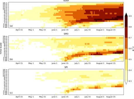
An example for the Northern Sierra, California PSA using summer average ERC is presented in
193
Figure 2 to guide the reader on the methods used to create subsequent Figures 3-7 based on drought
194
index time scale and lag. Maximum R2 (mapped in Figure 3) for EDDI (Figure 2a) is 0.86 at a 4-month
195
time scale (mapped in Figure 4) and a 0-day lag (mapped in Figure 5). Similarly, the maximum R2,
196
associated time scale, and associated lag for SPEI (Figure 2b) and SPI (Figure 2c) were mapped
197
spatially by PSA in Figure 3. The plume of higher correlations extending back from the end of August
198
indicates drought index memory in relation to fire danger (ERC in this case) and highlights potential
199
predictability of the fire-danger indices at the start of the season (1 June in this case). Start of season
200
maximum R2 was 0.50 for EDDI (Figure 2a), 0.40 for SPEI (Figure 2b), and 0.36 for SPI (Figure 2c),
201
and these are mapped spatially by PSA in Figure 6. Time scales associated with maximum start of
202
season R2 were 6-month (December-May) for EDDI, 12-month (June-May) for SPEI, and 11-month
203
(July-May) for SPI, and these are mapped spatially by PSA in Figure 7.
204
205
Figure 2: Average summer ERC correlated to (a) EDDI, (b) SPEI, and (c) SPI at the Northern Sierra
207
Nevada, California PSA. Vertical axis indicates drought index time scale in weeks (wk) or months (m)
208
and horizontal axis shows the drought index ending day for the correlation. The zero-day lag is
209
indicated at 31 August and the start of season lag (~90-day) is indicated at 1 June.
210
Maximum correlations between the four drought indices and seasonal ERC (summarized results
211
for 1000-hr fuel and 100-hr fuel shown in tables S1 and S2) are shown in Figure 3. Seasonally, only
212
minor variations in R2 were found with spring showing the strongest relationships (domain mean R2;
213
Table 1) for all drought indices. When considering CA-NV average R2 across all PSAs, the SPEI and
214
EDDI consistently show the strongest relationships (with the exception of winter, when SPI had a
215
greater R2 than EDDI) and often accounted for >80% of the ERC variance at individual PSAs, followed
216
by SPI. PDSI demonstrated the weakest relationships across all seasons.
217
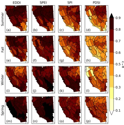
218
Figure 3: Maximum R2 of each drought index with the seasonal Energy Release Component (ERC)
219
fire danger index by season across the period 1979-2015 for each PSA in California and Nevada.
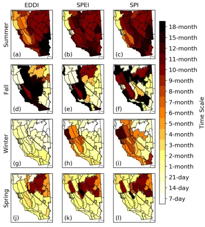
220
Overall, timescales of three to four months were most commonly associated with the maximum
221
correlations (Figure 4). Substantial variability can be found at the PSA level and also between
222
corresponded to 3- and 4-month time scales with EDDI (Figure 4d), but for SPEI (Figure 4e) maximum
224
correlations at many PSAs in central and northern California corresponded to 5-month to 7-month
225
timescales and to 2-month timescales in northern Nevada. In winter, maximum correlations
226
corresponded to 9-month and 10-month timescales for SPEI (Figure 3h) and SPI (Figure 4i) in several
227
central California PSAs.
228
229
230
Table 1. California-Nevada domain-average maximum R2 between seasonally averaged ERC and
231
drought indices.
232
Maximum R2 All Lags Maximum R2 90-day Lag
JJA
EDDI 0.76 0.44
SPEI 0.79 0.43
SPI 0.65 0.36
PDSI 0.56 0.30
SON
EDDI 0.76 0.21
SPEI 0.76 0.20
SPI 0.65 0.16
PDSI 0.48 0.10
DJF
EDDI 0.70 0.23
SPEI 0.82 0.24
SPI 0.75 0.23
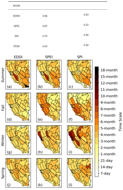
MAM
EDDI 0.86 0.29
SPEI 0.87 0.32
SPI 0.75 0.28
PDSI 0.63 0.20
233
Figure 4: Time scale of each drought index associated with the maximum correlations shown in Figure
234
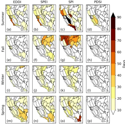
Lag times associated with maximum correlations to ERC (maximum correlations shown in
236
Figure 3) are shown in Figure 5. Generally, lags of less than 10 days were found with some variability
237
at the PSA level. Most notably lags of 30-70 days were found with SPI in northern CA-NV during the
238
fall.
239
240
Figure 5: Lag (in days) at which the maximum correlation (highest R2) is found between each of the
241
four drought indices (EDDI, SPEI, SPI, and PDSI) and the Energy Release Component (ERC)
fire-242
danger index, broken down by season and by PSA across California and Nevada.
243
Daily lag correlations revealed that maximum correlations almost always occurred within the
244
target season (lags < 90 days) and often close to the end of the target season. However, looking at the
245
lag correlations matrices revealed substantial memory in the drought indices with strong correlations
246
often beyond the 90-day lag. Figure 6 shows correlations for the 90-day (approximately one season)
247
lag to highlight potential windows of seasonal fire danger predictability by drought indices. Summer
248
showed the strongest correlations across the entire region with EDDI (domain mean R2 = 0.44) and
249
SPEI (domain mean R2 = 0.43) again most frequently having the highest R2. EDDI summer correlations
250
were strongest in California with several PSAs above 0.5 R2 and a peak of 0.59 at the Mid Coast to
251
with an R2 of 0.6, while R2 in most of central and northeast Nevada was above 0.5. Fairly strong
253
relationships were also found in spring with EDDI, SPEI, and SPI, but limited primarily to the
254
southernmost PSAs where several locations had R2 values between 0.5 and 0.59. Winter and fall
255
correlations were weak overall with the exception of a few PSAs where EDDI, SPEI, and SPI were
256
able to explain about 30-40% of the seasonal ERC variability.
257
258
Figure 6: Start of season (90-day lag) R2 of each drought index with the seasonal Energy Release
259
Component (ERC) fire danger index by season across the period 1979-2015 for each PSA in California
260
and Nevada.
261
Timescales associated with maximum 90-day lag correlations are displayed in Figure 7. Overall,
262
these timescales are much different than those shown in Figure 3, which primarily are associated with
263
much shorter lags. Summer correlations corresponded mostly to longer time scales of 10-15 months
264
for most PSAs. Notably shorter time scales were found in much of central and northern California
265
for EDDI and mostly northern coastal California for SPEI and SPI. For spring, the southern PSAs
266
mostly in the range of 1-3 months. Given the weak relationships found in fall and winter (Figure 6),
268
little value or physical meaning should be given to the associated time scales.
269
270
Figure 7: Time scale of each drought index associated with the 90-day lag correlations shown in Figure
271
5.
272
4.2. Evaporative demand attribution leading up to the Tubbs Fire
273
To illustrate the relationship of the drivers of E0 and developing fire potential, Figure 8 tracks
274
the development of the E0 anomaly and the contributions from each of its drivers across Sonoma
275
County, California from mid-August through the end of October, 2018, covering the period of eight
276
weeks prior to three weeks following the ignition of the Tubbs Fire. To minimize the noise of
day-to-277
day weather patterns, all variables are aggregated over a two-week window moving forward daily.
278
E0 is elevated above its climatological mean throughout the period, with two notable spikes of E0
279
percentiles elevated above 90% for extended periods. The first spike occurred from 31 August until 5
280
September (prior to the fire outbreak): its greatest early contribution was from above-normal
281
the time—particularly humidity, which remained above normal. During the first two weeks of
283
September, the above-normal temperatures abate, leading to a declining, though still positive, E0
284
anomaly. However, the mitigating effects of above-normal humidity and below-normal wind speeds
285
and solar radiation all reverse during this period to leave E0 near normal for the second half of
286
September. After this point, temperature remains near normal, but the combined effects of
now-287
below-normal humidity and above-normal wind speed and solar radiation dominate the E0 anomaly,
288
which climbs again through the day of the fire ignition (October 8) and afterwards. On the day of
289
ignition, E0 reaches its second spike when it exceeds its 95th percentile. This indicates that
near-290
surface moisture was decreasing and a drying of the air mass was taking place even during a period
291
of temperatures declining to near-normal values. It is also worth noting that wind speed had the
292
largest contributions during the onset of the second spike from 29 September through 2 October.
293
These patterns are suggestive of an important role of rapid (flash) meteorological impacts on fuels.
294
295
Figure 8: Attribution of evaporative demand (E0) anomaly prior to and during the Tubbs Fire in
296
Sonoma County, California, into contributions from each of its meteorological and radiative drivers.
297
The 2-week E0 anomaly (black line) is spatially averaged across Sonoma County. The contributions
298
from each of its drivers are shown as colored lines (temperature (T) in red, specific humidity (Q) in
299
blue, downwelling shortwave radiation (Rd) in purple, wind speed (U2) in green); percentiles of
2-300
week E0 are shown in dashed grey (right-hand axis); and the ignition date of the Tubbs Fire is shown
301
as a vertical brown line.
302
5. Discussion
303
Findings from the maximum correlation analysis (Figure 3) demonstrate that the multi-scalar
304
drought indices that incorporate E0 (EDDI and SPEI) typically have the strongest relationships to fire
305
danger indices. This is not a surprising finding given that fire danger indices are computed with the
306
same inputs as EDDI and SPEI, but it emphasizes an opportunity to take advantage of the
multi-307
scalar features of EDDI and SPEI to incorporate antecedent drought information into fire
308
daily derived indices. One exception to EDDI having the strongest relationships was winter when
310
SPI is better correlated than EDDI, which is most likely due to the fact that most of the annual
311
precipitation in the region (especially in California) falls during the winter. Precipitation is much
312
more limited during the warm-season months of April through September, and evaporative
313
dynamics--driven by high temperatures, high wind, and low humidity---have a greater effect on
314
drying of fuel moisture. The PDSI, which consistently showed the weakest relationships, also
315
incorporates E0 but uses a much different model than EDDI and SPEI to depict drought, and has a
316
static time scale of about 9-12 months that is clearly too long to reflect seasonal changes in fuel
317
moisture.
318
One application of drought indices that are strongly linked to fuel moisture is input for wildland
319
fire outlooks. In the United States, Predictive Services issues monthly a National Significant Wildland
320
Fire Potential Outlook [43] for fire management strategic planning and decision making. The drought
321
index lag correlations described here offer potential for informing fire outlook products. This is most
322
apparent in summer when EDDI and SPEI will likely provide the best results. A refinement of the
323
correlations could be to develop statistical regression models at the PSA level based on the best
324
combinations of drought indices to predict fuel moisture and fire potential. A combination of drought
325
indices is suggested since large variability was found when looking at individual PSAs and there was
326
not a single drought index “champion” for the entire region. A statistical model could help improve
327
summer outlooks given the poor skill currently found in seasonal dynamical precipitation forecasts
328
[44-47] and since precipitation plays only a minor role in fire danger during the summer in CA-NV.
329
The connection between E0 and fire danger indices also highlights the possibility of using seasonal
330
E0 forecasts as a tool for fire potential which have been shown to provide better skill than
331
precipitation forecasts in the U.S. [47].
332
Results from the E0 attribution highlight the potential to use this method as a tool to monitor
333
set-up conditions that are conducive to explosive fire growth and behavior as was seen with the
334
Tubbs Fire. Further examination of this methodology may show climatological signatures of fire
335
weather in E0 and its drivers that are typical to a particular region and season; this may prove to be
336
of predictive use to fire managers. Our correlation analysis focused on seasonal time scales but the
337
attribution example shows the potential for using E0 and EDDI and as a tool for guidance in
short-338
term products such as the Predictive Services’ 7-day Significant Fire Potential outlooks. Notably, the
339
drying of the air mass that began in mid-September and the steady increase in specific humidity
340
contributions (becoming the dominant driver several days before the fire began) to the E0 anomaly
341
combined with positive contributions from wind speed could be seen as an early warning signal for
342
increased fire potential when used in conjunction with many of the other indicators that were also
343
signaling extreme fire potential in the days leading up to the Tubbs Fire [28]. One case study greatly
344
limits the confidence in using this type of information for fire risk and more work is needed looking
345
at E0 and EDDI for prediction of short-term fire potential.
346
6. Conclusions
347
Strong relationships exist between all drought indices and fire danger indices tested at all
348
seasons and at most PSAs. Drought indices that incorporate E0 and are multi-scalar (i.e., EDDI and
349
SPEI) typically were found to have the strongest correlations to fire danger indices. This suggests that
350
will dryer fuel moisture and greater fire danger. Some predictive potential exists for start of season
352
fire potential outlooks using drought indices but is restricted to summer (entire region) and spring
353
(southern PSAs) with EDDI and SPEI providing the most value. Time scales associated with start of
354
season lag correlations indicate that antecedent drought conditions from the previous fall and winter
355
play a strong role in determining summer fuel moisture and fire danger in CA-NV.
356
To advance the understanding and value added of using drought indices for fire management,
357
real world testing and application is the next needed step. A partnership between Predictive Services
358
in northern California and the team of researchers who conducted this study has been established,
359
and beta-testing of EDDI as a management tool was performed during summer and fall of 2018. Initial
360
feedback indicates that EDDI was useful in determining set-up conditions prior to the Carr Fire (23
361
July), near Redding, California, and Camp Fire (8 November) in Paradise, California [48,49]. Both
362
fires were among the top 20 largest in California history and the Camp Fire was by far the most
363
destructive in history with 85 deaths and nearly 19,000 structures destroyed [13]. Two specific
364
applications of EDDI included using operational EDDI maps to replace the U.S. Drought Monitor
365
(USDM) [50] in U.S. Forest Service Region 5 severity funding requests (requests are made throughout
366
each fire season during periods with potential for abnormally severe fire behavior) and use of EDDI
367
graphics in North Ops Predictive Services’ seasonal fire potential outlooks. The USDM does not
368
explicitly consider fire potential and was not designed to be used operationally by fire managers, but
369
project stakeholders consistently pointed to using the USDM as the primary tool to assess drought
370
conditions related to fire potential. This is largely due to lack of training or engagement describing
371
proper tools that more accurately depict drought relationships to fire potential at various time scales.
372
This project highlights a value of connecting drought researchers to the fire management community.
373
Several web-based applications have been developed recently that can provide CONUS-wide
374
access to drought and fire danger indices in near real-time including the Google Earth Engine [51]
375
cloud computing tool Climate Engine [52], the West Wide Drought Tracker [53], and NOAA’s
376
operational EDDI tools [54]. These tools can be used with guidance from this analysis and feedback
377
from stakeholders to build the drought-fire connection capacity in the CA-NV DEWS. Further studies
378
in other regions, more research linking short-term drought (i.e., sub-monthly drought index time
379
scales) to real-time fire potential (i.e., flash drying of fuels) and behavior, and applied stakeholder
380
testing outside of northern California is needed and encouraged to successfully expand the
381
application of drought information for operational fire management purposes.
382
383
Supplementary Materials: The following are available online at www.mdpi.com/xxx/s1, Table S1:
California-384
Nevada domain-average maximum R2 between seasonally averaged 1000-hr fuel moisture and drought indices,
385
Table S2: California-Nevada domain-average maximum R2 between seasonally averaged 1000-hr fuel moisture
386
and drought indices.
387
388
Author Contributions: Conceptualization, D.M., T.B., and T.W.; Data Analysis and Visualizations, D.M. and
389
M.H.; Writing, Reviewing, and Editing, D.M., M.H., T.B., K.V., T.W., J.H., and M.S.; Stakeholder Engagement,
390
D.M., T.B., K.V., and T.W.
391
392
Funding: Funding for the work was provided by the National Oceanic and Atmospheric Administration and
393
National Integrated Drought Information System (NIDIS) Sectoral Applications Research Program grant
394
Acknowledgments:
396
Conflicts of Interest: The authors declare no conflict of interest.
397
References
398
1. Swetnam, T. W.; Betancourt, J. L. Fire-Southern Oscillation relations in the southwestern United States.
399
Science, 1990, 249(4972), 1017-1020.
400
2. Bessie, W. C.; Johnson, E. A. The relative importance of fuels and weather on fire behavior in subalpine
401
forests. Ecology, 1995, 76(3), 747-762.
402
3. Westerling A.L.; Brown, T.J.; Gershunov A.; Cayan D.R.; Dettinger M.D. Climate and wildfire in the
403
western United States. Bull Amer Meteor Soc., 2003, 84(5), 595-604. doi:10.1175/BAMS-84-5-595.
404
4. Littell, J. S.; McKenzie, D.; Peterson, D. L.; Westerling, A. L. Climate and wildfire area burned in western
405
US ecoprovinces, 1916–2003. Ecol Appl, 2009, 19(4), 1003-1021.
406
5. Riley, K.L.; Abatzoglou, J.T.; Grenfell, I.C.; Klene, A.E.; Heinsch, F.A. The relationship of large fire
407
occurrence with drought and fire danger indices in the western USA, 1984–2008: The role of temporal scale.
408
Int J Wildland Fire, 2013, 22(7), 894-909.
409
6. Prein, A. F.; Holland, G. J.; Rasmussen, R. M.; Clark, M. P.; Tye, M. R. Running dry: The US Southwest's
410
drift into a drier climate state. Geophys Res Lett, 2016, 43(3), 1272-1279.
411
7. Dennison, P. E.; Brewer, S. C.; Arnold, J. D.; Moritz, M. A. Large wildfire trends in the western United
412
States, 1984–2011. Geophys Res Lett, 2014, 41(8), 2928-2933.
413
8. Griffin, D.; Anchukaitis, K. J. How unusual is the 2012–2014 California drought? Geophys Res Lett, 2014,
414
41(24), 9017-9023.
415
9. Hatchett, B. J.; Boyle, D. P.; Putnam, A. E.; Bassett, S. D. Placing the 2012–2015 California-Nevada drought
416
into a paleoclimatic context: Insights from Walker Lake, California-Nevada, USA. Geophys Res Lett, 2015,
417
42(20), 8632-8640.
418
10. Robeson, S. M. Revisiting the recent California drought as an extreme value. Geophys Res Lett, 2015, 42(16),
419
6771-6779.
420
11. Shukla, S.; Safeeq, M.; AghaKouchak, A.; Guan, K.; Funk, C. Temperature impacts on the water year 2014
421
drought in California. Geophys Res Lett, 2015, 42(11), 4384-4393.
422
12. Williams, A. P.; Seager, R.; Abatzoglou, J. T.; Cook, B. I.; Smerdon, J. E.; Cook, E. R. Contribution of
423
anthropogenic warming to California drought during 2012–2014. Geophys Res Lett, 2015, 42(16), 6819-6828.
424
13. Cal Fire Top 20 Largest California Wildfires. Available online at:
425
https://www.fire.ca.gov/communications/downloads/fact_sheets/Top20_Acres.pdf (accessed on 27
426
December 2018)
427
14. Keeley, J. E.; Safford, H.; Fotheringham, C. J.; Franklin, J.; Moritz, M. The 2007 southern California wildfires:
428
lessons in complexity. J Forest, 2009, 107(6), 287-296.
429
15. Brown, J. F.; Wardlow, B. D.; Tadesse, T.; Hayes; M. J.; Reed, B. C. The Vegetation Drought Response Index
430
(VegDRI): A new integrated approach for monitoring drought stress in vegetation. GIScience & Remote
431
Sensing, 2008, 45(1), 16-46.
432
16. Sohrabi, M.M.; Ryu, J.H.; Abatzoglou, J.T.; Tracy J. Development of soil moisture drought index to
433
characterize droughts. J Hydrol Eng, 2015, 20(11), 04015025.
434
17. Carrão, H.; Russo, S.; Sepulcre-Canto, G.; Barbosa, P. An empirical standardized soil moisture index for
435
18. Anderson, M.C.; Norman, J.M.; Mecikalski, J.R.; Otkin, J.A.; Kustas, W.P. A climatological study of
437
evapotranspiration and moisture stress across the continental United States based on thermal remote
438
sensing: 2. Surface moisture climatology. J Geophys Res-Atmos, 2007, 112(D11).
439
19. Vicente-Serrano, S. M.; Beguería, S.; López-Moreno, J. I. A multiscalar drought index sensitive to global
440
warming: the standardized precipitation evapotranspiration index. J Climate, 2010, 23(7), 1696-1718.
441
20. Hobbins, M.T; Wood, A.W.; McEvoy, D.J.; Huntington, J.L.; Morton, C.; Anderson, M.C.; Hain, C.R. The
442
Evaporative Demand Drought Index: Part I – linking drought evolution to variations in evaporative
443
demand. J Hydrometeorol, 2016, 17, 1745-1761.
444
21. McEvoy, D.J.; Huntington, J.L.; Hobbins, M.T.; Wood, A.W.; Morton, C.; Anderson, M.C.; Hain, C.R. The
445
Evaporative Demand Drought Index: Part II – CONUS-wide assessment against common drought
446
indicators. J Hydrometeorol, 2016, 17, 1763-1779.
447
22. Abatzoglou, J. T.; Kolden, C. A. Relationships between climate and macroscale area burned in the western
448
United States. Int J Wildland Fire, 2013, 22(7), 1003-1020.
449
23. Predictive Services website. Available online at: https://www.predictiveservices.nifc.gov. (accessed on 4
450
February 2019)
451
24. Pulwarty, R., and J.P. Verdin (2013), Crafting early warning systems: the case of drought. In Measuring
452
Vulnerability to Natural Hazards: Towards Disaster Resilient Societies, Birkmann, J., United Nations University
453
Press, Tokyo.
454
25. Eidenshink, J.; Schwind, B.; Brewer, K.; Zhu, Z. L.; Quayle, B.; Howard, S. A project for monitoring trends
455
in burn severity. Fire Ecol, 2007, 3(1), 3-21.
456
26. Balch, J.; Schoennagel, T.; Williams, A.; Abatzoglou, J.; Cattau, M.; Mietkiewicz, N.; St Denis, L. Switching
457
on the Big Burn of 2017. Fire, 2018, 1(1), 17.
458
27. Nauslar, N.; Abatzoglou, J.; Marsh, P. The 2017 North Bay and Southern California Fires: A Case Study.
459
Fire, 2018, 1(1), 18.
460
28. Abatzoglou, J. T. Development of gridded surface meteorological data for ecological applications and
461
modelling. Int J Climatol, 2013, 33(1), 121-131.
462
29. Palmer, C. P. Meteorological drought. US Weather Bureau research paper, 1965, 45.
463
30. Heim, R. R. Computing the monthly Palmer Drought Index on a weekly basis: A case study comparing
464
data estimation techniques. Geophys Res Lett, 2005, 32(6).
465
31. Allen, R. G.; I. A. Walter; R. Elliott; T. Howell; D. Itenfisu; M. Jensen. The ASCE standardized reference
466
evapotranspiration equation, 2005, Rep. 0-7844-0805-X, 59 pp
467
32. McKee, T. B.; Doesken, N. J.; Kleist, J. The relationship of drought frequency and duration to time scales.
468
In (Vol. 17, No. 22, pp. 179-183), Proceedings of the American Meteorological Society, Boston, MA, United
469
States, January, 1993.
470
33. Ford, T.W.; Labosier, C.F. Meteorological conditions associated with the onset of flash drought in the
471
eastern United States. Agr Forest Meteorol, 2017, 247, 414-423.
472
34. Otkin, J.; M.D. Svoboda; E. Hunt; T. Ford; M. Anderson; C.R. Hain; Basara, J. Flash droughts: A review and
473
assessment of the challenges imposed by rapid onset droughts in the United States. Bull Amer Meteor Soc.,
474
2017, 99(5), 911-919.
475
35. Lorenzo-Lacruz, J.; Vicente-Serrano, S. M.; López-Moreno; J. I., Beguería, S.; García-Ruiz, J. M.; Cuadrat, J.
476
M. The impact of droughts and water management on various hydrological systems in the headwaters of
477
36. McEvoy, D.J.; Huntington, J.L.; Abatzoglou, J.T.; Edwards, L. An evaluation of multi-scalar drought indices
479
in Nevada and eastern California. Earth Interact, 2012, 16, 1-18.
480
37. Abatzoglou, J.T.; Barbero, R.; Wolf, J.; Holden, Z. Tracking interannual streamflow variability with drought
481
indices in the U.S. Pacific Northwest. J Hydrometeorol, 2014, 15, 1900–1912.
482
38. Vicente-Serrano, S. M.; Beguería, S.; Lorenzo-Lacruz, J.; Camarero, J. J.; López-Moreno, J. I.; Azorin-Molina,
483
C.; ... Sanchez-Lorenzo, A. Performance of drought indices for ecological, agricultural, and hydrological
484
applications. Earth Interact, 2012, 16(10), 1-27.
485
39. Hao, Z.; AghaKouchak, A. A nonparametric multivariate multi-index drought monitoring framework. J
486
Hydrometeorol, 2014, 15(1), 89-101.
487
40. Farahmand, A.; AghaKouchak, A. A generalized framework for deriving nonparametric standardized
488
drought indicators. Adv Water Resour, 2015, 76, 140-145.
489
41. Deeming, J.E.; Burgan, R.E.; Cohen, J.D. The National Fire Danger Rating System – 1978. USDA Forest
490
Service, Intermountain Forest and Range Experiment Station, General Technical Report INT-39, 1977.
491
42. Hobbins, M.T., The variability of ASCE Standardized Reference Evapotranspiration: a rigorous,
CONUS-492
wide decomposition and attribution. Trans. ASABE, 2016, 59(2), 561-576.
493
43. Garfin, G.M.; Brown, T. J.; Wordell, T.; Delgado, E. The making of national seasonal wildfire outlooks. In
494
Climate in Context: Science and Society Partnering for Adaptation. Parris, A.S.; Garfin, G.M.; Dow, K; Meyer,
495
R.; Close, S.L. John Wiley and Sons Ltd.: West Sussex, UK, 2016; Volume 1, pp. 143-172.
496
44. Yuan, X.; Wood, E. F.; Roundy, J. K.; Pan, M. CFSv2-based seasonal hydroclimatic forecasts over the
497
conterminous United States. J Hydrometeorol, 2013, 26, 4828-4847.
498
45. Saha S., and coauthors. The NCEP Climate Forecast System Version 2. J. Climate, 2014, 27, 2185-2208.
499
46. Wood, E.; Schubert, S.; Wood, A.; Peters-Lidard, C.; Mo, K.; Mariotti, A.; Pulwarty, R. Prospects for
500
advancing drought understanding, monitoring and prediction. J Hydrometeorol, 2015, 16.
501
47. McEvoy, D. J.; Huntington, J. L.; Mejia, J. F.; Hobbins, M. T. Improved seasonal drought forecasts using
502
reference evapotranspiration anomalies. Geophys Res Lett, 2016, 43(1), 377-385.
503
48. Wachter, B. (Predictive Services, Redding, California, United States). Personal communication, 2018.
504
49. Wachter, B. Applied EDDI. FIRESCOPE Fall Meeting, San Diego, California, November 8, 2018. Available
505
online at: https://drive.google.com/file/d/1X-efCp6UDPlMj11W55m1MfinvYsKPA_S/view?usp=sharing.
506
(accessed on 4 February 2019)
507
50. Svoboda, M.; LeComte, D.; Hayes, M.; Heim, R.; Gleason, K.; Angel, J.; ... Miskus, D. The drought monitor.
508
Bull. Amer. Meteor. Soc., 2002, 83(8), 1181-1190.
509
51. Gorelick, N.; Hancher, M.; Dixon, M.; Ilyushchenko, S.; Thau, D.; Moore, R. Google Earth Engine:
510
Planetary-scale geospatial analysis for everyone. Remote Sens Environ, 2017, 202, 18-27.
511
52. Huntington, J. L.; Hegewisch, K. C.; Daudert, B.; Morton, C. G.; Abatzoglou, J. T.; McEvoy, D. J.; Erickson,
512
T. Climate Engine: cloud computing and visualization of climate and remote sensing data for advanced
513
natural resource monitoring and process understanding. Bull Amer Meteor Soc, 2017, 98(11), 2397-2410.
514
53. Abatzoglou, J. T; McEvoy, D. J.; Redmond, K. T. The west wide drought tracker: drought monitoring at
515
fine spatial scales. Bull Amer Meteor Soc, 2017, 98(9), 1815-1820.
516
54. Evaporative Demand Drought Index website. Available online at: https://www.esrl.noaa.gov/psd/eddi/.
517
(accessed on 4 February 2019)