Separation of the elastic waves’ system in pre-stretched bar devices
Gr´egory Haugoua, Nicolas Leconte, and Herv´e Morvan
Laboratory of Industrial and Human Automation Control, Mechanical Engineering and Computer Sciences, UMR CNRS 8201, University of Valenciennes, Le Mont-Houy, France
Abstract. The loading mode generated by Kolsky bars apparatus is limited due to physical reasons to a duration time of around 0.4 ms. This is not suited in the characterization of high ductility metallic alloys up to fracture at moderate strain rates, since the duration time is too short. The pre-stretched bar device is a good candidate to characterize these materials up to the moderate strain rates. Unfortunately, the elastic waves are generally not separated in time at measurements points in the input bar, and post treatment leads to assumptions. A configuration of the pre-stretching conditions that ensures no superposition of the elastic waves’ system developed along the input bar is thus proposed so as to fulfill standard data analysis requirements, i.e. without any assumptions. However, a drawback of the proposed device is that one of its hydraulic devices generates a loosen tail. This statement comes from a FE numerical model of the whole set-up including the generation of the loosen tail. Finally, an analytical correction to cancel the loosen tail is proposed and validated with respect to a numerical model featuring ideal pre-loading conditions.
1. Introduction
The loading generated by Kolsky bars apparatus – developed in the 50s’ either for tension or compression loadings – is transient by nature since it is generated by the impact of a striker on a incident bar [1–3]. Since the length of the striker is 1 m at most due to technical reasons, the duration of the pulse generated by the metallic striker is generally limited to 0.4 ms, excepted for tension tests using a long U-shape projectile [4]. Indeed, the duration time depends on the ratio between the length of the striker and the wave speed of the elastic pulse generated just after impact. For instance, for a strain rate aimed at 100/s and for a duration time of 0.4 ms, the total strain cannot exceed 0.04. Therefore, it is generally admitted that Kolsky bars cannot be employed or adapted in order to characterize high ductility metals up to fracture at moderate strain rates. The pre-stretched bar technique allows to load specimens with upper duration times than those generated by strikers. To the knowledge of the authors’, the first device of this kind has been developed by Albertini [5]. Note that the ratio between the pre-stretched part and the input bar is 0.75 in this version, so as to maximize the duration time. This ratio became more or less a standard ratio to be used with this kind of set-up. The duration times of the pre-stretched technique are commonly found to be between 2 and 4 ms [2,5–9]. For instance, with a duration time of 1.2 ms, it is possible to reach a strain rate of 160/s for a total strain of 0.2. Thanks to these durations, it is possible to reach moderate rates of strain that can be divided at least by 3 when compared to Kolsky bars. However, a major drawback in the use of pre-stretched bars is that the incident pulse is cancelled by the aCorresponding author:
-30 -20 -10 0 10 20 30
-1 000 -800 -600 -400 -200 0 200 400 600 800 1 000
0 1 2 3 4 5 Load (k
N)
E
lastic strai
n
(
µµ
str
a
in
)
Time (ms)
input bar signal - G2 output bar signal - G3 pre load force - G1
Loosen tail
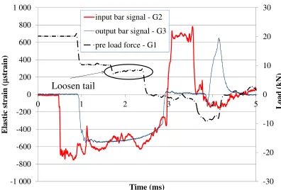
Figure 1.Typical recording of a tensile test using a pre-stretched bar with superposition of the elastic waves’ system (20 MnCr5 rounded specimen at 100/s – pre-stretched length of 5556 mm).
arrival of the reflected one and cannot be obtained without approximations in the post processing [8]. In fact, it is due to a superposition of the elastic waves’ system in the input bar. By the way, the signals can still be exploited by rebuilding the incident signal [2,5–9]. The rebuilt incident pulse is considered to be valid and representative of the expected one by some authors. The shape of the incident pulse is still subjected to discussions (Fig.1).
To the authors’ knowledge, none of the presented devices [2,4–9] allows avoiding both the superposition of the elastic waves’ system and the existence of an intrinsic tail. The aim of the article is thus to propose a pre-stretched bar set up for the fast dynamics loading of high ductility metals, which does not feature a superposition of the elastic waves’ system. In fact, the aim is to be able to benefit from the advantages of such loadings modes (long duration time) without the corresponding drawbacks (superposition of the elastic waves’ system), i.e., being
2990 7512
3793 566
F
A B
G2 D E
G3
G
D E
5552
G1
6976
x
Figure 2.Pre-stretched tensile bar and sample – in mm.
Table 1.Properties of the input and output bars.
C (m/s) E (GPa) ν Input/output bars 4612 163.5 0.3
able to post-process the waves in a standard way. It is foreseen that it can be achieved by suitably setting the ratio between the pre-stretched part and the length of the input bar. However, since the development of this kind device is not straightforward [10], the authors propose to couple the experiments together with numerical simulations in order to validate some assumptions, conclusions, and technical choices. Europlexus software [11] is used to perform the numerical simulations. It’s based on a finite-element computer program for the analysis of fluid-structure systems subjected to transient dynamic loadings. Europlexus software is being jointly developed by the French Commissariat `a l’Energie Atomique (CEA – Saclay) and by the Joint Research Centre of the European Commission (JRC – Ispra).
The article is organized as follows. The pre-stretched bar device proposed and its corresponding numerical model are presented in Sect. 2. In Sect. 3, the results obtained from the experiments are compared to the numerical model. Finally, a correction in the raw signals analysis provided by the set-up is proposed and validated with respect to the numerical model given in Sect. 4.
2. Pre-stretched device and its modeling
2.1. Loading principle
A sketch of the Split Hopkinson Tension Bar installed in 2006 at L.A.M.I.H. laboratory, France, is given in Fig.2.
Here, the tensile testing scenario consists of partly pre-stretching (A to B, here 2990 mm in length) the input bar (A to D), which length is 7512 mm. The length of the output bar (E to G) is 6976 mm. Note that both bars were obtained from the same cast process (Table1).
Both bars have an average diameter equal to 10.98 mm and are precisely aligned and guided on a rigid I-frame. The specimen is inserted between positions D and E using M7 threads. The pre-loading force F – stabilized between A and B – is generated by means of two quasi-static loadings applied on the input bar:
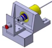
• A locking mechanism based on an hydraulic jack (Max. capacity: 600 kN) ensures the fastening of the input bar thanks to a brittle fuse, which geometric details are given in Fig.3.
• After being fixed using the locking mechanism, the input bar is pre-stretched using another hydraulic
Figure 3.Locking mechanism placed in B – Details of the fuse system.
Figure 4.Pre-stretched bar mechanism placed in A.
device composed by a hydraulic hollow cylinder (Max. capacity: 300 kN), as illustrated in Fig. 4. The pre-load force is recorded on a full strain bridge bonded at 5552 mm from the specimen (position G1). The force value is limited to 45 kN so as to keep the pre-stretched part of the input bar in its elastic domain and to avoid any risk of sliding inside the locking system.
The combination of these two operations ensures the storage of an elastic energy that can be brutally released when the brittle fracture of the fuse occurs at the position B. Then, an incident elastic wave in tension develops with a rise-time of about 26µs thanks to a specific design of the connectors mounted on the fuse (Fig.3). The elastic wave propagates along the input bar with a constant duration time depending on the length of the pre-stretched part, and loads the specimen up to fracture. A set of two additional full strain bridges (HBM LY 41 350–length: 1.5 mm) are strategically positioned along the experimental set-up for the post-treatment of the waves (see Sect.2.3):
– The position of gauge G2 (Fig.2) is defined to detect both incident and reflected waves separately.
– The gauge G3 (Fig. 2) is placed to measure the transmitted signal.
Here, the position in B is chosen so that no superposition of the reflected wave with the incident one can occur at the position of the strain gauge bonded in G2. The strain rate value can be changed by varying the pre-loading force F of the pre-stretched device. Note that to evaluate the proposed configuration; rounded specimens made of 20 MnCr5 material are tested in the next experiments.
2.2. Finite element modeling
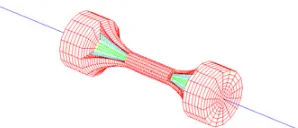
Figure 5. Mesh of the rounded specimen fixed between the cylindrical bars.
while a simple approach is employed for the modeling of the specimen, since the focus of this work is based on the development of a configuration where no superposition of the elastic waves occurs.
The experimental device is respectively modeled by 7512 (input bar) and 6976 (output bar) 1-D bar elements. The material behaviour of the bars is considered to be elastic (see Table1). Note that the connections between 1-D bar elements (at points D and E, Fig.2) and the faces of the specimen consisting of 3-D hexahedral elements are exactly imposed on the corresponding node velocities by means of Lagrange multipliers (Fig.5) [12].
The boundary conditions are imposed on the set up as follows:
– an initial stress condition is imposed in the bar elements corresponding to the stretched part of the input bar,
– an unilateral constraint is imposed at the beginning of the input bar (point A) by means of pinballs (one attached to the ground and one massless attached to the input bar) in order to prevent the motion of the bar in the positive x-direction (Fig.2).
Finally, the bar elements of the numerical model corresponding to the strain gauges bonded on the experimental set up at positions G1 to G3 are chosen as “numerical gauges” in order to ensure a similar post-treatment for both experiments and numerical simulations. The specimen consists of 9408 fully-integrated 3-D hexahedral finite elements (Fig.5). Its material behaviour is modeled by a Ludwik law (where A=750 MPa, B= 820 MPa and n=0.525 at a strain rate of 300/s). The failure is simply predicted by means of element erosion when a threshold von Mises stress is reached.
2.3. Elastic waves’ analysis
The strain gauges are commonly used to measure the elastic strain waves propagating along the bars (commonly called incident, reflected and transmitted pulses). Gauge G2 is used to detect incident and reflected pulses, while gauge G3 is used to measure the transmitted pulse. These measurements are required to calculate the current velocities and forces at interfaces, and stress/strain engineering relations based on the one-dimensional elastic wave theory [13,14]. The incident elastic wave propagates along the input bar with a constant velocity and square shape. Its amplitude is function of the pre-stretched force value applied on the input bar. When the incident pulse reaches the specimen, it is partly reflected towards the input bar, and partly transmitted along the output bar after crossing throughout the specimen. The amplitudes of the
incident, reflected, and transmitted pulses depend on the mechanical and geometrical properties of the specimen, so that the gauge section is calibrated to balance reflected and transmitted pulses. It is assumed that the specimen, which is short enough in comparison with the input and output bars, reaches a state of forces’ equilibrium after several reflections of elasto-plastic waves inside its gauge length. The following equations are used to compute the global values as a function of time, and are based on the elastic pulses namedεinc(t),εref(t),εref(t)assuming that a separation of the elastic waves in time is ensured:
VO B(t)=CO B·[εtr a(t)] (1)
VI B(t)=CI B·[εi nc(t)+εr e f(t)] (2) where VOB(t) and VIB(t) are the output and input bars velocities associated to the wave’s speeds COB and CIB, respectively.
FO B(t)=SO B·EO B·[εtr a(t)] (3)
FI B(t)=SI B·EI B·[εi nc(t)+[εr e f(t)] (4) where FOB(t) and FIB(t) are output and input bars forces associated to the elastic moduli EOB and EIB and cross sections SOB and SIB, respectively. The average engineering stress and the engineering strain rate are presented in relations (5) and (6), respectively:
σeng(t)= EO B·SO B
S0 ·
[εtr a(t)] (5)
˙
εeng(t)= VI B(t)−VO B(t)
L0
(6) where S0 and L0 are respectively the initial cross section and length in the gauge zone. Plastic strains are determined as a function of time using a first order integration of strain rate relation (6).
The validity of the data analysis presented above is based on two hypotheses. First, the stresses and velocities are assumed to propagate through the bars without dispersion. If this first hypothesis is true, a linear relation between the diameter of the bar and the pulse amplitude is fulfilled. Secondly, the time required by the elastic wave to propagate through the specimen must be short compared to the total time of the test; in these conditions, many reflections inside the specimen are produced. Note that these equations are regardless used in the data analysis process of the experiments (Sect. 2.1) and of the finite element approach (Sect.2.2).
3. Typical responses
3.1. Experiments
-30 -20 -10 0 10 20 30
-1 000 -800 -600 -400 -200 0 200 400 600 800 1 000
0 1 2 3 4 5 Load (k
N)
E
lastic
strai
n
(
µµ
str
a
in
)
Time (ms)
input bar signal - G2 output bar signal - G3 pre load force - G1
Loosen tail
Figure 6. Typical recording of a tensile test using the pre-stretched bar without superposition of the elastic waves’ system (20 MnCr5 rounded specimen tested at 300/s – pre-stretched length of 2990 mm).
avoided since the incident wave reveals a quasi-constant amplitude when compared to Fig.1. These conditions are in accordance with the classical data analysis employed for Kolsky bars apparatus. The post-treatment presented in Sect.2.3can thus be used without any assumption. The main goal of this work has thus been achieved.
However, a drawback of the proposed set up is that it generates a loosen tail. It starts in the current experiment at around 1.5 ms and it is highlighted in the force signal recorded at gauge G1 by red dotted lines (Fig.6). In fact, some observations using high speed imaging have revealed that this phenomenon may be generated when releasing the hydraulic system used to pre-stretch the input bar (Point A, Fig.2). The loosen tail is directly detected in the gauge G1 used for the measurement of the pre load force applied on the input bar. As observed in the input signal of Fig.6, the loosen tail is also detected at gauge G2 once the incident pulse decreases to zero, and the consequences on the amplitude of the reflected wave are not negligible. In the space-time diagram (not shown here for the sake of conciseness), the loosen tail and its effects on the elastic waves’ system can be observed easily. In fact, it affects the shape of the reflected single and therefore the strain, strain rate and input force expressions given by relations 2, 4 and 6. Note that for a longer pre-stretched part, this problem is delayed due to the position of the point of measurement of the incident and reflected waves.
In classical configurations of Kolsky bars, a separation in time of the incident pulse with the reflected pulse is intrinsic. However, a tail can be generated between the incident and reflected pulses due to imperfections in the loading conditions or/and in the material properties of the bars [15]. Here, the authors have highlighted the existence of a typical tail for pre-stretched bar devices obtained under tensile testing conditions (Fig.6).
3.2. FEM results
First, it is important to highlight that the model presented in Sect.2.2is ideal, i.e., it does not take into account any spurious effect that could be produced by the hydraulic device placed in A (Fig. 2). An additional boundary condition is thus introduced at this location in the numerical model to this end. A force is thus added in the
30
15
0
-10
-25
0 0.5 1 1.5 2 2.5 3 3.5
Force (kN)
Time (ms)
Figure 7a.Typical responses recorded at position of strain gauge G1 considering tail effects (elastic prediction in red, experiment in black, and computation in blue).
1500
1000
500
0
-500
-1000
-1500
0 0.5 1 1.5 2 2.5 3 3.5
microstrain
Time (ms)
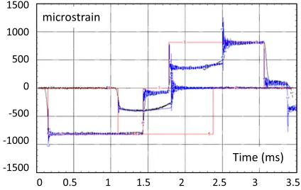
Figure 7b. Typical responses recorded at position of strain gauges G2 and G3 considering tail effects (elastic prediction in red, experiment in black, and computation in blue).
FE model at the hydraulic device location (in A). Note that the amplitude of the tail depends on the pre-load force value. Its time-expression for a pre-load force of 25 kN (see Sect. 3.1) needs to be defined in the numerical model. To do so, it is proposed to identify the loosen tail based on the force signal recorded at gauge G1 (Fig. 6). It is assumed that a second order polynomial is suited to model the loosen tail [16]. A least square approach is employed to identify its coefficients. On the one hand, the force-time expression of the loosen tail is fully identified at gauge G1, and on the other hand, the phenomenon generating it is supposed to be located at the beginning of the input bar (point A). It is thus necessary to shift the identified expression in time. The time shift is simply obtained from the wave speed in the input bar and the distance between the strain gauge G1 and point A. The results – summarized in Figs. 7a,b – compare theoretical elastic predictions, the experimental results, and the computations. A good agreement is observed between the computations and the signals recorded experimentally. It can thus be concluded that:
– Europlexus software provides accurate predictions of elastic waves’ propagation principle.
– The birth place of the loosen tail is located at point A, – The loosen tail is entirely generated by the hydraulic
Figure 8.Tail correction effect on reflected pulse.
– The methodology employed to generate the loosen tail at its birth place in the numerical model is correct.
4. Analytical correction of the loosen tail
4.1. Correction of the typical responses
A methodology to correct the tail identified previously (Sect. 3.2) that is similar to the one dedicated to the correction of the tail of Kolsky bars is proposed. In the typical loading conditions of the pre-stretched input bar, the reflected signal (and thus the material laws identified when post-processing these signals, see Sect. 2.3) is affected by the loosen tail. Thus, it must be corrected so as to fulfill the relation (7):
In Sect. 3.2 the profile of the loosen tail has been accurately identified at gauge G1. The tail recorded at gauge G2 is thus similar to the one identified at gauge G1 according to 1D elastic wave propagation theory, but is cut by the reflected wave. Consequently, the reflected wave is underestimated and the tail is used to correct the reflected signal according to the developments of Gary [16]. It is then simply subtracted on the raw signals (red curve in Fig.8). Finally, the Eq. (7) must be checked after applying the correction.
Note that this correction is based on empirical observations and must be confirmed with respect to the achievement of forces’ equilibrium assuming that the amplitude of the transmitted pulse is not modified by the tail. To do so, that, the authors propose to determine a typical strain-stress curve based on:
– the determination of the reflected wave from incident and transmitted signals,
– the determination of the transmitted signal from the incident and reflected signals,
– no tail correction is applied on the reflected signal as described in Fig.8.
It is then clearly put into evidence the consequences of the loosen tail on a typical material response. In Fig.10 are presented the results of the different means to calculate the strain-stress relation according relation given in (7).
In details, the loosen tail affects directly the reflected signal thus the strain rate and strain values (see Eq. (2) and (6)) and given in Fig.10. Indeed, a correction of the
0 200 400 600 800 1 000 1 200 1 400
0.00 0.05 0.10 0.15 0.20 0.25 0.30
T
ru
e str
ess
(MP
a
)
True strain (.)
Tail correction Reflected rebuilt Transmitted rebuilt Without tail correction
Figure 9.Validation of the tail correction process for the stress-strain curves calculation.
-1200 -1000 -800 -600 -400 -200 0 200 400 600 800 1000
0.0 0.2 0.4 0.6 0.8 1.0 1.2 1.4 1.6
E
lastic
s
train
(
µµ
str
ain)
Time (ms)
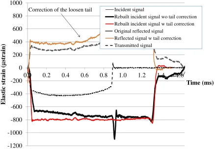
Incident signal
Rebuilt incident signal wo tail correction Rebuilt incident signal w tail correction Original reflected signal Reflected signal w tail correction Transmitted signal Correction of the loosen tail
Figure 10.Comparison of the (un)corrected incident signals (see relation. 7).
reflected signal reveals being unavoidable. It is confirmed by the fact that the determination of the reflected signal based on the incident and transmitted signals (see relation. 7) matches well with the tail correction process proposed here. Finally, the transmitted signal is correct because any modification will conduce to important errors in the strain-stress relations.
4.2. FEM verification and final results
30
15
0
-15
0 0.5 1 1.5 2 2.5 3 3.5
Force (kN)
Time (ms)
Figure 10a. Typical responses recorded at position of strain gauge G1 without tail effects (elastic prediction in red, experiment in black, and computation in blue).
1500
1000
500
0
-500
-1000
-1500
0 0.5 1 1.5 2 2.5 3 3.5
microstrain
Time (ms)
Figure 10b. Typical responses recorded at position of strain gauges G2 and G3. Experimental tail correction (elastic prediction in red, experiments in black, and computations in blue).
5. Conclusions
A principle based on a pre-stretched bar that ensures no superposition of the elastic waves’ system has been proposed together with a particular technical solution. This sort of experimental set-up is interesting in particular for the characterization of high ductility metallic alloys up to fracture at moderate strain rates. However, the selected technical solution generates a loosen tail initiated at the end of the incident pulse which induce a disturbance of the reflected pulse. A correction that allows recovering an ideal configuration has thus been proposed and validated with respect to a numerical model developed
using Europlexus software. Future works will focus on technological solutions avoiding the emergence of loosen tails. The numerical modeling approach of the device will be also used to investigate on other kinds of loadings. References
[1] H. Kolsky, “Stress waves in solids”, Dover Publica-tions Inc., New York, 1963.
[2] U.S. Lindholm, L.M. Yeakley, “Some experiments with the Split Hopkinson Pressure Bar”, Experimen-tal Mechanics, Vol.12, pp 317–355, 1964.
[3] W. Chen, B. Song, “Split Hopkinson (Kolsky) bar. Design, testing and Applications.” New York (USA): Springer; 2011.
[4] R. Gerlach, C. Kettenbeil, N. Petrinic, International Journal of Impact Engineering, Vol. 50, pp 63–67, 2012.
[5] C. Albertini, M. Montagnani, Mechanical Properties at High Strain Rates, Vol.21, pp 22–32, 1974. [6] Tore Børvik, Arild H. Clausen, Odd Sture
Hop-perstad, Magnus Langseth, International Journal of Impact Engineering, Vol. 30, Issue 4, pp 367–384, 2004.
[7] E. Cadoni, M. Dotta, D. Forni, N. Tesio, C. Albertini, Materials and Design, Vol.49, pp 657–666, 2013. [8] Y. Chen, A.H. Clausen, O.S. Hopperstad, M.
Langseth, International Journal of Impact Engineer-ing, Vol.38, Issue 10, pp 824–836, 2011.
[9] D. Saletti, S. Pattofatto, H. Zhao, Mechanics of Materials, Vol.65, pp 1–11, 2013.
[10] G. Riganti, E. Cadoni, Materials and Design, Vol.57, pp 156–167, 2014.
[11] http://www-epx.cea.fr/
[12] F. Casadei, N. Leconte. International Journal for Numerical Methods in Engineering,86(1), pp 1–17, 2011.
[13] J. Achenbach. (1973), “Wave propagation in elastic solids”. North-Holland.
[14] K. Graff. (1975), “Wave motion in elastic solids”. Ohio State University Press.
[15] H. Zhao, G. Gary, J.R. Klepaczko, International Journal of Impact Engineering, Vol. 19, n◦ 4, pp 319–330, 1997.