(will be inserted by the editor)
Modelling and Optimisation of Adaptive Foraging in Swarm
Robotic Systems
Wenguo Liu · Alan FT Winfield
Received: date / Accepted: date
Abstract Understanding the effect of individual parameters on the collective performance of swarm robotic systems in order to design and optimise individual robot behaviours is a significant challenge. This paper presents a macroscopic probabilistic model of adaptive collective foraging in a swarm of robots, where each robot in the swarm is capable of ad-justing its time threshold parameters following the rules described in (Liu et al, 2007). The swarm adapts the ratio of foragers to resters (division of labour) in order to maximise the net swarm energy for a given food density. A probabilistic state machine (PFSM) and a number of difference equations are developed to describe collective foraging at a macroscopic level. To model adaptation we introduce the new concepts of the sub-PFSM and private/public time thresholds. The model has been extensively validated with simulation trials, and results show that the model achieves very good accuracy in predicting the group performance of the swarm. Finally, a real-coded genetic algorithm is used to explore the parameter spaces and optimise the parameters of the adaptation algorithm. Although this paper presents a macroscopic probabilistic model for adaptive foraging, we argue that the approach could be applied to any adaptive swarm system in which the heterogeneity of the system is coupled with its time parameters.
Keywords macroscopic probabilistic modelling·swarm robotics·collective foraging
1 Introduction
In recent decades swarm intelligence (SI) has gained increasing attention as a bio-inspired approach to coordinating behaviours of groups of simple robots in multi-robot systems. Case studies include flocking/aggregation (Matari´c, 1995; Vaughan et al, 2000; Tanner et al, 2004; Dorigo et al, 2004; Garnier et al, 2008); collective clustering/sorting (Holland and Melhuish, 1999; Martinoli et al, 1999; Wilson et al, 2004); collective searching/inspection (Reif and Wang, 1999; Dudenhoeffer et al, 2001; Correll and Martinoli, 2009); cooperative transport/handling (Kube and Bonabeau, 2000; Ijspeert et al, 2001; Gross and Dorigo, 2004)
Wenguo Liu and Alan FT Winfield Faculty of Environment and Technology
and collective foraging (Krieger et al, 2000; Labella et al, 2006). Although there is no central controller governing the behaviour of the swarm and the robots themselves often have very limited sensing, communication and computation, complex collective behaviours emerge from local interactions among the robots and between the robots and the environment with relatively simple individual control rules. Systems based on the principles of SI, known also as swarm robotic systems, emphasise self-organisation and distributedness in a large number of robots. With homogeneity and simplicity as design goals at the individual unit level, the main advantages of the swarm approach lie in the properties of scalability, adaptivity and robustness. However, bottom-up design cannot provide us with quantitative prediction of the swarm performance. In order to design and optimise individual robot behaviours, and hence achieve the desired collective swarm properties, we need to understand the effect of individual parameters on the group performance. Real robot experiments and simulations are the most direct way to observe the behaviour of the system with different parameters. However, trials with real or simulated robots do not scale well as the size of the system grows. It is therefore impractical to search the whole design parameter space to find the best solutions using a trial and error approach.
Mathematical modelling and analysis offers both an alternative and complement to ex-periments and simulation, and attention has been direction in recent years to addressing the modelling problem in swarm robotics using probabilistic approaches. One such approach is macroscopic modelling, which aims to directly describe the overall collective behaviour of the system. One of the fundamental elements of the macroscopic probabilistic model are the Rate Equations, which have been successfully applied to a wide variety of problems in physics, chemistry, biology and the social sciences. For instance, Sumpter and Pratt (2003) developed a general framework for modelling social insect foraging systems with gener-alised rate functions (differential equations). Sugawara and coworkers (Sugawara and Sano, 1997; Sugawara et al, 1999) first presented a simple macroscopic model for foraging in a group of communicating and non-communicating robots, with analysis under different con-ditions. Lerman and Galstyan (2001, 2004) proposed a more generalised and fundamental contribution to macroscopic modelling in multi-agent systems. Lerman et al (2001) devel-oped a macroscopic model of collaborative stick-pulling, and the results of the macroscopic model quantitatively agree with both embodied and microscopic simulations. Lerman (2002) presents a mathematical model of foraging in a homogeneous multi-robot system to under-stand quantitatively the effects of interference on the performance of the group. Agassounon et al (2004) used the same approach to capture the dynamics of a robot swarm engaged in collective clustering.
Rather than using a time-continuous model, Martinoli and coworkers (Martinoli et al, 2004) considered a more fine-grained macroscopic model of collaborative stick-pulling which takes into account more of the individual robot behaviours, in the discrete time do-main, using difference equations. They suggest that time-discrete models are the most appro-priate solution for the level of description characterised by logical operators and behavioural states. Similarly, Correll and Martinoli (2005) used a macroscopic probabilistic model for analysis of beaconless and beacon-based strategies for a swarm turbine inspection system, and to find an optimal collaboration policy minimising the time to completion and the overall energy consumption of the swarm in Correll and Martinoli (2006). In Winfield et al (2008) the same macroscopic modelling approach has been applied to study a swarm of wireless networked robots in which the movements of the robots are no longer constrained within a bounded environment.
excep-tion of the work of (Lerman et al, 2006), which extended the macroscopic probabilistic model to distributed robots that adapt their behaviour based on estimates of the global state of the system. In this work robots engaged in a puck collecting task need to decide whether to pick up red or green pucks based on observed local information. The model must therefore take into account the heterogeneities in the robot population. Lerman, et al, claim that the model can be extended to other systems in which robots use a history of local observations of the environment as a basis for making decisions about future actions.
In our previous work (Liu et al, 2007), we presented a simple algorithm for a group of foraging robots which try to maximise the net swarm energy, through adaptive division of labour. Individual robots each have the same threshold-based controllers and two time thresholds are used to regulate the behaviour of the robots, either foraging or resting. Three adaptation cues (internal, social and environmental), based on local sensing and communi-cations, dynamically vary the time spent foraging or resting. The adaptation algorithm has a number of parameters which are used to adjust the contribution of each cue. Simulation results show the adaptation mechanism is able to guide the swarm towards energy efficiency. However, with a set of parameters selected by hand it is not clear that the swarm has the best performance it can achieve, and there are no obvious guidelines for manually finding the optimal parameters. To address these problems we will develop a macroscopic probabilistic model of adaptive foraging to investigate the effect of the individual parameters of the adap-tation mechanisms on the performance of the system. In general, the probabilistic modelling approach is built upon the finite state machine of the individual controller and deals with two types of transitions: one happens when certain external conditions are true (transition probabilities based), the other relies on internal time parameters (threshold based). Unlike the model described in (Lerman et al, 2006), where the adaptation mechanism adjusts the state transition probabilities directly, we will consider a different and complementary case in which the adaptive process tunes two determinstic time parameters of the robot controller using more complex adaptation rules. The main challenge of applying the macroscopic prob-abilistic modelling framework to adaptive foraging lies in the nested dynamic introduced by the time thresholds. Once the model has been developed and validated, we can then use it to optimise the design of the adaptation algorithm.
This paper is organised as follows: Section 2 introduces the collective foraging scenario and our adaptation algorithm. Section 3 develops the macroscopic probabilistic model of collective adaptive foraging in detail. We first outline the steps of such an approach, then explain the derivation of difference equations for each state in the probabilistic finite state machine. Section 4 validates the model using simulation trials for a range of different exper-iments. A real-coded genetic algorithm is then used to find the optimal parameters for the adaptation algorithm. Finally section 5 concludes the paper.
2 Adaptive collective foraging
homing scanarena grabfood
leavinghome deposit
movetohome movetofood
resting randomwalk
at home
success close to food
success
T2> Tr in search area
find food find food
lost food T1> Ts
T1> Ts
scan time up T1> Ts
[image:4.595.101.417.82.185.2]at home
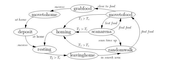
Fig. 1: The threshold-based robot controller for collective foraging, with adaptive division of labour.
time the robot spends searching and is set when the robot moves out of state resting; T2
is set when the robot moves to state resting and counts the time resting in the nest. The transitions from states randomwalk, scanarena, or movetofood to state homing are triggered whenever searching time T1reaches its threshold Ts; such a transition will reduce the number
of foragers which in turn minimises the interference caused by overcrowding. The transi-tion between states resting and leavinghome, is triggered when the robot has rested for long enough, i.e. T2≥Tr, will drive the robot back to work to collect more food for the colony,
which means increasing the number of foragers in the swarm. Note that to keep the diagram clear, with the exception of state resting, the robot can transition from any state to state avoidance — not shown in Figure 1 — whenever obstacles are detected; after the collision avoidance behaviour is completed the robot will return to its previous state.
The individuals in the swarm use three adaptation cues: internal cues (successful or un-successful food retrieval); environmental cues (collision with other robots while searching) and social cues (teammate food retrieval success or failure) to dynamically regulate the two internal thresholds. This adaptation is based on the following rules:
Tsi(k+1) =T i
s(k)−α1Ci(k) +β1Psi(k)−γ1Pif(k) (1)
Tri(k+1) =Tri(k) +α2Ci(k)−β2Psi(k) +γ2Pif(k)−ηRi(k) (2)
where i indicates the ID for each robot, Ci(k)counts the contribution from environmental cues, Psi(k)and Pif(k)for social cues, and R
i(k)for internal cues. The adjustment factors
α1,α2,β1,β2,γ1,γ2andη, whose values are positive real numbers, are used to moderate
the contribution of each corresponding cue. Note that the adjustments take place only when certain state transitions happen (or in state resting). In most cases, the contribution of each cue is zero. Ci(k), Ri(k), Psi(k)and Pif(k)are defined below.
Ci(k) =
(
1 state randomwalk→state avoidance
0 otherwise (3)
Ri(k) =
1 state deposit→state resting −1 state homing→state resting 0 otherwise
Psi(k) =
0 not in resting state
SPs(k) state deposit→state resting
∑N
j=1,j6=i{Rj(k)|Rj(k)>0}in resting state
(5)
Pif(k) =
0 not in resting state
SPf(k) state homing→state resting
∑N
j=1,j6=i{|Rj(k)||Rj(k)<0}in resting state
(6)
where SPsand SPfrepresent social cues (food retrieval success and failure respectively),
defined as follows:
SPs(k+1) =SPs(k)−δ+ N
∑
i=1
(Ri(k)|Ri(k)>0) (7)
SPf(k+1) =SPf(k)−δ+ N
∑
i=1
(|Ri(k)||Ri(k)<0) (8)
Attenuation factorδ is introduced here to simulate gradual decay rather than instantly dis-appearing social cues. Note that as the social cues are only accessible for the robots in the nest, two categories of robots will be affected. One group are those already resting in the nest, the other are those ready to move to state resting from states homing or deposit; the former can ‘monitor’ the change of social cues and then adjust time threshold parameters, while the latter will benefit from the gradually decaying cues left by teammates. The two situations for updating Pi
s(k)and Pif(k)are shown in Equations (5) and (6).
3 A probabilistic model for adaptive foraging
For most behaviour-based robotic systems, although the behaviour of a particular robot at a given time is fully determined, the transitions from one state (behaviour) to another exhibit some probabilistic properties over time within the population of the swarm. The central idea of macroscopic probabilistic modelling is to describe the system as a series of stochastic events and use rate equations to capture the dynamics of these events. A general approach to developing a macroscopic probabilistic model for swarm robotic systems can be summarised as follows:
step 1 describe the behaviour of the individual robots of the swarm as a finite state machine (FSM);
step 2 transform the FSM into a probabilistic finite state machine (PFSM), describing the swarm at a macroscopic level;
step 3 develop a system of rate equations for each state in the PFSM, to describe the chang-ing average number of robots between states at a macroscopic level;
step 4 measure the state transition probabilities using experiments with one or two real robots, or estimate them using analytical approaches, and then
step 5 solve the system of rate equations.
continuous time or discrete time. Clearly the complexity of the model depends very much on the task itself. Consider our adaptive foraging scenario: the goal of the swarm is to maximise the net energy of the swarm, but this metric is directly coupled with the number of robots either Resting or non-Resting. The probabilistic model is capable of capturing the dynamics of the average transitions of robots between states, thus if we can embed the adaptation rules into the general probabilistic model, the relationship between the low-level parameters (i.e. adjustment factors of the adaptation rules) and the group metric (net swarm energy) will be expressed mathematically.
3.1 The probabilistic finite state machine
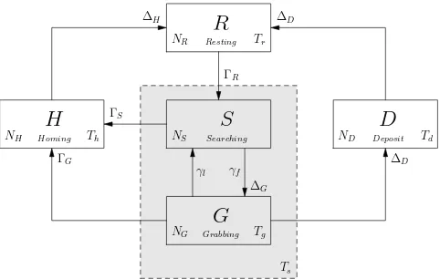
The foraging controller FSM for an individual robot shown in Figure 1 can be described as a PFSM for the whole swarm as shown in Figure 2. To reduce the complexity of the model, the nine states of the FSM have been simplified to five: states movetohome and Deposit in the FSM correspond to state Deposit in the PFSM; states leavinghome, randomwalk and scanarena in the FSM correspond to state Searching; states movetofood and grabfood in the FSM correspond to state Grabbing, states Resting and Homing in the FSM remain the same. Note that (with the exception of state Resting), each of these PFSM states also includes robots in state Avoidance, as in the FSM.
S
NS Searching
G
NG Grabbing Tg
R
NR Resting Tr
D
ND Deposit Td
H
NH Homing Th
γf γl
∆D
∆G ΓS
ΓG
ΓR
∆H ∆D
[image:6.595.125.366.342.495.2]Ts
Fig. 2: Probabilistic finite state machine for adaptive collective foraging. Each block rep-resents the state and the average number of robots in that state, denoted NX. The number
of robots transferring from one state to another is marked withΓ and∆;∆G,∆Dand∆H
represent the total number of robots moving into states G, D and H respectively;ΓSandΓG
represent the number of robots moving from state S and G. All transitions, with the excep-tion of those marked withγl andγf, have transition probability 100% but are delayed by
some time period. Note that the two transitions from states S and G to H are functions of time Ts, while the transition from G to D is a function of time Tg. Note also that Tgis a nested
time parameter.
move towards the target food-item until it is close enough to grab it. Once the robot success-fully grabs the food-item after Tgtime steps, it will move to state Deposit, D. After the robot
deposits the food-item, it will stay in state Resting, denoted R, for Tr time steps and then
return to state Searching. Alternatively, if a robot in state S fails to find a food-item within the search time Ts, it will move to state Homing, denoted H. The same rule applies to a robot
in state G if its searching time limit is reached, even though the robot is moving towards a food-item. Because of competition among robots if more than one robot catches sight of the same food-item clearly only one of them can actually grab it; a robot in state G therefore has probabilityγlto lose sight of the food-item because it has been already grabbed by another
robot, which in turn causes the robot to return to state Searching. Note that robots in states G, H and D, are all moving towards a specific target which is either a food-item or the nest, hence Tg, Thand Tdrepresent the average times that the robot will stay in those states; these
are not design parameters (as Tsor Tr), but have been estimated based on simple
[image:7.595.129.362.300.431.2]geometri-cal considerations and robot control strategies, as outlined in the Appendix. Table 1 lists the primary notation used in the paper.
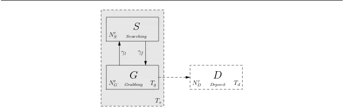
Table 1: Key to the primary notation used in the PFSM and macroscopic model
notation description
NX number of robots in state X, X∈ {S,G,D,H,R}
∆X total number of robots moving into state X
ΓX number of robots moving into state Homing from state X
M number of food-items available in the environment γl probability to lose sight of a food-item
γf probability to find a food-item
γr probability to collide with other robots
Tg average grabbing time
Th average homing time
Td average deposit time
Tx(y) private time threshold, x∈ {r,s}, y∈ {h,d,s}
Tx public time threshold
3.2 Rate equations
Let NS(k), NG(k), ND(k), NH(k)and NR(k)be the average number of robots in states
Searching, Grabbing, Deposit, Homing and Resting respectively, at time step k. As the total number of robots in the swarm must remain constant from one time step to the next, if N0
represents the total number of robots in the swarm, then we have
N0=NS(k) +NR(k) +NG(k) +ND(k) +NH(k) (9)
The changes in the average number of robots in each state can be described with a set of difference equations in the discrete-time domain. Consider NS(k)first, the number of robots
in state Searching at time step k+1 can be expressed as
NS(k+1) =NS(k) +γl(k)NG(k) +ΓR(k+1)−γfM(k)NS(k)−ΓS(k+1) (10)
losing sight of a food-item for one robot,γl(k), varies from time to time depending on the
number of food-items available and the number of robots competing for food. The third term
ΓR(k+1)is the number of robots moving from state Resting to state Searching at time step
k and will be explained in section 3.4.2. The remaining terms describe the number of robots moving from state Searching to other states:γfM(k)NS(k)denotes those transferring to state
Grabbing, in which M(k)is the number of food-items available in the environment at time step k andγf denotes the probability that one robot finds a food-item while searching in the
arena. We define there to be, on average, pnewnew food-items growing in the arena each time
step (Liu et al, 2007). As a robot can only grab one food-item at a time, the total number of food-items collected by the robots is equivalent to the number of robots transferring to state Deposit at time step k, denoted with∆D(k), thus we have
M(k+1) =M(k) +pnew−∆D(k) (11)
The final entry on the RHS of Equation (10),ΓS(k+1), represents the number of robots
transferring to state Homing from state Searching. Similarly, for state Grabbing:
NG(k+1) =NG(k) +γfM(k)NS(k)−γl(k)NG(k)−∆D(k+1)−ΓG(k+1) (12)
WhereΓG(k)counts those robots failing to grab food-items as they run out of searching time
and therefore transfer to state Homing. For state Deposit:
ND(k+1) =ND(k) +∆D(k+1)−∆D(k−Td) (13)
For state Homing:
NH(k+1) =NH(k) +∆H(k+1)−∆H(k−Th) (14)
For state Resting,
NR(k+1) =NR(k) +∆D(k−Td) +∆H(k−Th)−ΓR(k+1) (15)
Where
∆H(k+1) =ΓS(k+1) +ΓG(k+1) (16)
∆D(k+1) =∆G(k−Tg)−ΩG(k−Tg)ΛG(k; Tg) (17)
∆G(k+1) =γfM(k)NS(k) (18)
ΩG(k−Tg)in Equation(18) represents that number of robots transferring to state Grabbing
from state Searching at time step k−Tg, whose remaining searching time credit is
insuf-ficient to allow those robots to grab the food-item successfully. This group of robots will move to state Homing once their searching time is up during the next Tg time steps (from
k−Tg to k).ΛG(k; Tg)denotes the fraction of robots successfully grabbing the food-item
at time step k after spending Tgsteps moving towards it. It is equivalent to the probability
that no transition from state Grabbing to state Searching is triggered during the time interval
[k−Tg+1,k], and can be expressed as follows:
ΛG(k; Tg) =
k
∏
i=k−Tg+1
S
N′
S Searching
G
N′
G Grabbing Tg
D
N′
D Deposit Td
γf
γl
[image:9.595.71.418.80.191.2]Ts
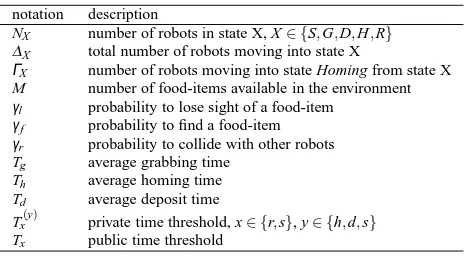
Fig. 3: sub-PFSM for robots engaged in the “searching-grabbing” task. The sub-PFSM in-cludes states Searching and Grabbing, and models only a sub-set of robots in the swarm. At each time step a new instance of the sub-PFSM is formed and each instance has a limited lifetime. During its lifetime, robots may exit the sub-PFSM to state Deposit.
3.3 A sub-PFSM for the “searching-grabbing” task
To solve Equations (10) to (18), we need to derive equations forΓS,ΓG,ΓRandΩG. As shown
in Figure 2,ΓS,ΓG andΩG(related to∆D) are all related to the searching time threshold
Ts. There is no straightforward way of writing down these equations explicitly, as in the
previous section, because of the nesting of time parameters (Tsand Tg). Assume a group of
robots transfer to state Searching at time 0, then after Ts steps, some robots may move to
state Deposit between time steps Tgand Ts, the others then move to state Homing at time step
Ts+1. Clearly, within time Ts, these robots can only be in the states Searching, Grabbing and
Deposit. Once we known how these robots are distributed across these three states over time, the number of robots moving to state Homing, i.e.ΓSandΓG, can be obtained. Based on these
considerations we introduce a sub-PFSM which includes two states for task “searching-grabbing”, as shown in Figure 3. The “searching-grabbing” task is clearly a part of the overall foraging PFSM of Figure 2, hence we refer to it as a sub-PFSM.
At each time step one new instance of the sub-PFSM is formed with a different initial number of robots in state Searching, which were transferred from state Resting in the pre-vious time step. The sub-PFSM can be identified by its date of birth (DOB), i.e. the time that it is formed. Because of the searching time threshold the sub-PFSM will no longer ex-ist after these robots transfer to other states some time steps later. During the limited-time lifecycle of a sub-PFSM, its subset of robots could split into states Searching or Grabbing, or move into state Deposit after spending Tg steps in state Grabbing. Thus we can develop
rate equations to capture the change in number of robots in the states within the sub-PFSM from one time step to the next.
To avoid confusion with the previous notation of the rate equations, let NS′(k; i)be the
number of robots in state Searching in the sub-PFSM, and NG′(k; i)for state Grabbing, where
i indicates the DOB of the PFSM, and k represents the current time step for the sub-PFSM (as in the full sub-PFSM). A mathematical description for the sub-sub-PFSM of Figure 3 can then be developed as follows
NS′(k+1; i) =NS′(k; i) +γl(k)NG′(k; i)−γfM(k)NS′(k; i) (20)
NG′(k+1; i) =NG′(k; i) +γfM(k)NS′(k; i)−γl(k)NG′(k; i)
−∆G′(k−Tg; i)ΛG(k; Tg)
Where∆G′(k−Tg; i)ΛG(k; Tg)counts the number of robots that will be successfully
trans-ferred to state Deposit.ΛG(k; Tg)is obtained through Equation(19).∆G′(k; i)represents the
number of robots moving to state Grabbing (in the sub-PFSM) at time step k, where
∆′
G(k+1; i) =γfM(k)NS′(k; i) (22)
The initial conditions for the sub-PFSM are NS′(i; i) =ΓR(i), NG′(i; i) =0.
Although only one sub-PFSM is formed each time step, each sub-PFSM can have dif-ferent lifetimes because of the adaptation rules (to be discussed in the next section), hence there could be more than one sub-PFSM coming to the end of its life cycle at time step k. To obtain the number of robots that transfer to state Homing,ΓSandΓG, we need to to know
which sub-PFSMs expire at time step k. LetS(k)denote the collection of all the DOBs for
all of those sub-PFSMs, then we have
ΓS(k) =
∑
i∈S(k)
NS′(k; i) (23)
ΓG(k) =
∑
i∈S(k)
NG′(k; i) (24)
ΩG(k−Tg) =
k
∑
m=k−Tg
∑
i∈S(m)
∆′
G(k−Tg; i) (25)
3.4 Modelling of adaptation rules
At this stage the PFSM model is almost complete, but requires the description ofΓR(k)
and the newly introducedS(k). Clearly these two variables have close links with the two
time thresholds Tsand Tr. For a swarm with fixed time thresholds, i.e. no adaptation,
de-riving equations forΓR(k)andS(k)is straightforward. That isS(k) ={k−Ts}andΓR(k) =
∆D(k−Td−Tr) +∆H(k−Th−Tr). However for the case with adaptation, a robot in the
swarm may change its time threshold parameters based on internal, social or environmental cues over time, thus Tsand Tr are no longer fixed and indeed highly dynamic. Equations
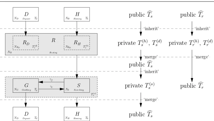
(1) and (2) show a linear adjustment operation for the time threshold parameters from each cue. The contribution of each cue is proportional to the number of robots transferring into corresponding states, e.g the contribution of environmental cues equals the average number of robots moving into state Avoidance (not shown in the PFSM but included in state Search-ing). Although the macroscopic model doesn’t itself take the difference between individual robots into account, the sub-PFSM models a subset of robots in the PFSM. It is therefore practical to introduce exclusive time thresholds into the sub-PFSM and apply the adaptation rules to these robots and their time thresholds. The exclusive time thresholds owned by each instance of the sub-PFSM are called private time thresholds. In consequence two public time thresholds, owned by all robots, are introduced into the model to link many of these private ones. The private time thresholds play the role of deciding when the transition from one state to another is triggered, while the public time thresholds are used to accumulate the contributions from all the adaptation cues which have been applied to the swarm. They affect each other in a bi-directional manner, and are described as follows.
3.4.1 Private and public time thresholds
‘merge’ ‘inherit’
‘merge’ ‘inherit’ ‘merge’ ‘inherit’
S
NS Searching
R
NR Resting
RH
NRH T
(h) s
RD
NRD T
(d) s
D
ND Deposit Td
H
NH Homing Th
G
NG Grabbing Tg
D
ND Deposit Td
H
NH Homing Th
publicTcs
privateTs(h),Ts(d)
publicTcs
privateTs(s)
publicTcs
publicTcr
privateTr(h),Tr(d)
publicTcr γf
γl
[image:11.595.72.414.78.271.2]T(s) s
Fig. 4: Relationship between private and public time thresholds. Pseudo states RDand RH
represent the robots moving from state Deposit and Homing respectively, each is paired with one private resting time and one private searching time. The lifetime of the private searching time is decided by the lifetime of the paired private resting time threshold, e.g. Ts(h)paired
with Trh. The influence domain of each time threshold is separated with dotted lines.
Resting into two groups according to which states they transferred from: either state Homing or Deposit, marked as pseudo-states RHand RDas shown in Figure 4. Two private resting
time thresholds Tr(d)and T(
h)
r , corresponding to the robots that transferred from state Deposit
and Homing respectively, are introduced into the model. In the same way as those in the sub-PFSMs, each subset of robots which move to state Resting will have their own copy of private resting time threshold Tr(d)or Tr(h). The transitions from state Resting to Searching
are decided by these two private resting time threshold parameters. Three private searching time thresholds, Ts(h), Ts(d)and Ts(s), are introduced for the pseudo-states (RHand RD) and
the sub-PFSM. Among these three private searching time thresholds, Ts(h)and Ts(d)are used
to track the contribution of social cues when the robots are in state Resting, while Ts(s)is
used to track the contribution of environmental cues. The transitions from state Searching and Grabbing to Homing are now determined by Ts(s). Clearly, each of these private time
thresholds has a limited lifetime. They are created when a certain fraction of robots move to a specific state and destroyed once those robots move to a new state. During their life cycles, their values will be updated according to the adaptation rules. Like the sub-PFSMs, they can be identified with DOBs. For example, the notation Tr(d)(k; i)is used to represent
the values of private resting time threshold at time step k, where i indicates the time step that this private resting time threshold is formed (its DOB). Using this notation, S(k)in
Equations (23) to (25) can be expressed as
S(k) =i|k−1−i<Ts(s)(k−1; i)∧k−i>Ts(s)(k; i) (26)
where k−i represents the time steps elapsed from the DOB until step k.
To obtainΓR(k), letRH(k)andRD(k)represent the collection of DOBs for the private
cycles at time step k, then
ΓR(k) =
∑
i∈RH(k)
∆H(i−Th) +
∑
i∈RD(k)
∆D(i−Td) (27)
Clearly,RH(k)andRD(k)can be expressed similar toS(k)
RH(k) =i|k−1−i<Tr(h)(k−1; i)∧k−i>Tr(h)(k; i) (28)
RD(k) =i|k−1−i<Tr(d)(k−1; i)∧k−i>Tr(d)(k; i) (29)
As each of the private time thresholds has a limited life cycle and is attached to separate fractions of robots, a public searching time thresholdTbsand a public resting time threshold
b
Trare introduced to help model the adaptation rules applied on the swarm. Figure 4 depicts
the relationship between the private and public time thresholds. Each private time threshold has its own influence domain. The public time thresholds are mainly used to accumulate the contribution of corresponding private time thresholds to the swarm. Although they have no direct influence on the transitions from one state to the another, they decide the initial values of the private time thresholds. To link the private and public time thresholds, two operations, ‘inherit’ and ‘merge’, are defined here. The private time thresholds ‘inherit’ the up-to-date public time threshold when they are formed, and will update (‘merge’ into) the corresponding public time threshold at the end of their lifetime based on certain rules. For resting time thresholds, one pair of ‘inherit’ and ‘merge’ operations is applied. While for searching time thresholds the adjustments first take place on Tshand Tsdwhen robots move
into and stay in state Resting, in the same way as for the resting time thresholds, then the adjustments continue on Ts(s)when robots are in the states of the sub-PFSM. Two pairs of
‘inherit’–‘merge’ operations are necessary for the adjustments of searching time threshold.
3.4.2 Modelling adaptation of time thresholds
To complete the model a mathematical description of the private time thresholds Ts(s), Tr(d)
and Tr(h)needs to be developed. Following the considerations above, this section gives a
detailed derivation of private resting time thresholds Tr(d) and Tr(h). The private searching
time threshold Ts(s)can be obtained using the same approach and is detailed in Liu (2008).
As shown in Equation (2), the adjustment of resting time threshold falls into three cat-egories corresponding to the contribution from internal cues, social cues and environmental cues respectively. The internal cues and social cues are applied whenever the transitions to state Resting occur; then, the social cues continue to play a role while the robots are in state Resting. The environmental cues take effect only for robots in state Searching. To embed these three cues into the model they must be dealt with separately.
A. Internal cues & social cues
When the robots move to state Resting at time step i a new copy of private resting threshold, either Tr(h)or Tr(d)according to which state they have transferred from, is created
and will be destroyed when that fraction of robots leaves state Resting. As depicted in Figure 4, the mathematical modelling of private resting time thresholds can be summarised in three phases, as follows:
As soon as the robots move into state Resting, a private resting time threshold is formed for these robots with the initial value of public resting time threshold. According to Equa-tions (4) to (6), the internal cues will be applied to adjust the private resting time threshold first, followed by the social cues. Following Equation (2), we have
Tr(h)(k+1; k+1) =Tbr(k)−β2SPs(k) +γ2SPf(k) +η (30)
Tr(d)(k+1; k+1) =Tbr(k)−β2SPs(k) +γ2SPf(k)−η (31)
whereβ1,β2,γ1andγ2are the adjustment factors for social cues, andηis the adjustment
factor for internal cues. SPs(k)and SPf(k) represent the social cues of the swarm. The
first term in the RHS of Equations (30) and (31) represents the ‘inherit’ operation from the public resting time threshold. The second and third terms in the RHS count the contribution of social cues. The final term then denotes the adjustment of internal cues.
For SPf(k)and SPs(k), according to Equations (7) and (8), we have
SPf(k+1) =SPf(k)−δ+∆H(k−Th) (32)
SPs(k+1) =SPs(k)−δ+∆D(k−Td) (33)
whereδ is the attenuation factor, while ∆H(k−Th)and∆D(k−Td)denote the increased
value of social cues respectively, following Equation (4). phase 2) when robots are in state Resting
As shown in the final rows of Equations (5) and (6), social cues continue to play a role in adjusting the time thresholds when robots are in state Resting, thus we have
Tr(h)(k+1; i) =T(
h)
r (k; i)−β2∗∆D(k−Td) +γ2∗∆H(k−Th) (34)
Tr(d)(k+1; i) =Tr(d)(k; i)−β2∗∆D(k−Td) +γ2∗∆H(k−Th) (35)
phase 3) when robots move to state Searching
Once the resting robots move into state Searching, a merge operation will be applied to update the public resting time threshold. At each time step there may be more than one sub-set of resting robots running out of resting time. In order to calculate the contribution that the private resting time thresholds make to the public resting time thresholdTbr, we need
to know:
– the number of robots which leave state Resting in the current time step, and
– the impact of social cues and internal cues on the private resting time thresholds Tr(h)
and Tr(d)during their lifecycles.
The contribution of each fraction of reactive robots (from state Resting to Searching) to the public resting time threshold can be expressed as the product of the number of robots and the change of the corresponding private resting time threshold. Let∆
Tr(h) and∆Tr(d) be the
total contribution provided by the resting robots transferring from state Homing and Deposit respectively, then
∆T(h)
r (k) =
∑
i∈RH(k)
∆H(i−Th)
(Tr(h)(k; i)−Tbr(i−1))
(36)
∆T(d)
r (k) =
∑
i∈RD(k)
∆D(i−Td)
(Tr(d)(k; i)−Tbr(i−1))
WhereRD(k)andRH(k)are defined in Equation (28) and (29).
B. Environmental cues
The environmental cues adjust the resting time threshold when robots move from state Searching to Avoidance. Although the change of resting time threshold in this case will not affect the behaviour of the robots until they return home, they make contributions to the public resting time thresholdTbr. This contribution can be expressed asα2γrNS(k), whereα2
is the adjustment factor,γris the probability that one robot will collide with another robot
when searching for food, andγrNS(k)is the number of robots moving into state Avoidance
at time step k.
C. Updating ofTbrfrom all cues
Combining the effect of all cues, the public resting threshold Trwill be updated as
fol-lows
b
Tr(k+1) =Tbr(k) +
∆T(h)
r (k) +∆Tr(d)(k) +α2γrNS(k)
N0
(38)
Where N0is the total number of robots in the swarm.
3.5 The swarm net energy consumption
Now that we have described collective adaptive foraging mathematically using the above equations, the metric of the system – the net energy income of the swarm – can be expressed accordingly. Assume each robot will consume Er units of energy in state Resting, and Es
units of energy in all other states, each time step. Moreover, assume that one collected food-item will deliver the swarm with Ecenergy units. If E(k)denotes the net energy income for
the swarm at time step k, then we have
E(k+1) =E(k) +Ec∆D(k−Td)−ErNR(k)−Es(N0−NR(k)) (39)
Where Ec∆D(k−Td)denotes the energy collected by the robots, while ErNR(k)and Es(N0−
NR(k))represent the energy consumed by the robots, in each time step.
4 Results – validation and optimisation
Using geometrically estimated transition probabilities (γf,γr andγl) and time parameters
(Tg, Th and Td), whose derivation is outlined in the Appendix, our mathematical model of
adaptive collective foraging can be solved approximately using a computer aided numerical analysis approach. This section presents the validation of the mathematical model and uses the model to optimise the adjustment factors.
4.1 Validation of the model
Rinner ψv
Rv
Rh
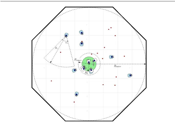
[image:15.595.71.412.78.318.2]Router
Fig. 5: Screenshot of the simulation for collective foraging. The home region, with radius Rh
(0.5 m), is located in the centre of a bounded arena. The food-items will ‘grow’ randomly within the annular region between radius Rinner(0.7 m) and radius Router(3.0 m).
centre of the arena and indicated with a grey colour. This is where each robot deposits food-items collected and rests before resuming its search. A light source in the nest acts as a homing beacon for robots. Each robot has physical dimensions 0.26m×0.26m and is equipped with three front mounted light intensity sensors for homing, one at the centre and two on either side, 60◦from centre. The robot senses it is at home with a floor facing colour sensor. The food-items scattered in the arena are small marked boxes which can be sensed – from a distance – by the robot’s front facing camera. The robot processes the image from its camera in order to determine the relative angle between its current heading to the location of the food-item, then turns, moves forward to the target and, when close enough, grabs it with its gripper. As the robot cannot sense its distance to the target, the grippers are equipped with two beam sensors which are triggered whenever a food-item is directly in-between the two paddles of the gripper. The robot is also equipped with three front mounted infra-red (IR) proximity sensors for detecting collisions with other robots or the arena wall (the food-items cannot be sensed by the IR sensors). The robot’s physical parameters are given in Table 2.
4.1.1 case 1: Pnew=0, no adaptation
We first consider a canonical foraging scenario, widely used in robotics research, in which no adaptation takes place. Initially there are 40 food-items randomly scattered in the arena. The task of the swarm is to collect all food-items and to deposit them in the home region. The time parameters τs and τr are set to 100 seconds and 0 seconds respectively in the
simulation. As the time step duration is set to 0.25 seconds, we fix Ts=400 and Tr=0 in the
Table 2: Robot and Environment parameters for simulation and probabilities estimation
Parameters Value Description
V 0.15 m/s Robot forward velocity
w1 15◦/s Robot rotation velocity to face food-item
w2 15◦/s Robot rotation velocity to face home
ψv 60◦ View angle of camera
ψb 95◦ Proximity sensor detection angle
Rv 2 m Camera detection range
Rb 0.4 m Proximity sensor range
Rp 0.13 m Robot body radius
Rh 0.5 m Radius of home region
Rinner 0.7 m Inner boundary radius of food growing area
Router 3 m Outer boundary radius of food growing area
Er 1 unit/s Energy consumed per second in state Resting
Es 10 units/s Energy consumed per second in non-Resting state
Ec 2000 units Energy delivered per food-item
∆t 0.25 s Time step duration
tl 2 s Gripper loading time
δ 0.1 Attenuation factor of social cues
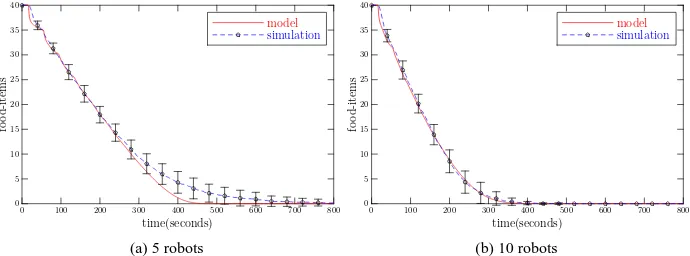
are set to the values given in Table 2. We vary the population of the swarm from 3 to 20 and repeat each simulation run 40 times. In parallel, we run the macroscopic probabilistic model with corresponding parameters and initial conditions.
0 5 10 15 20 25 30 35 40
fo
o
d
-i
te
m
s
0 100 200 300 400 500 600 700 800 time(seconds)
model simulation
(a) 5 robots
0 5 10 15 20 25 30 35 40
fo
o
d
-i
te
m
s
0 100 200 300 400 500 600 700 800 time(seconds)
model simulation
[image:16.595.76.421.366.494.2](b) 10 robots
Fig. 6: Comparison of simulated and modelled instantaneous food-items uncollected in the arena, with different swarm sizes. Initially there are 40 food-items randomly scattered in the arena. The error bars show the standard deviation of 40 simulation runs.
2008), it is not surprising to see that in some cases the model is less quantitatively accurate (although still qualitatively correct).
100 200 300 400 500 600 700 800
co
m
p
le
te
ti
m
e
(s
ec
on
d
s)
0 2 4 6 8 10 12 14 16 18 20 swarm size
model simulation
(a) food collected = 80%
100 200 300 400 500 600 700 800
co
m
p
le
te
ti
m
e
(s
ec
on
d
s)
0 2 4 6 8 10 12 14 16 18 20 swarm size
model simulation
[image:17.595.74.426.144.272.2](b) food collected = 90%
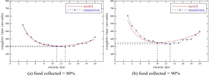
Fig. 7: Comparison of simulated and modelled time to collect 80% (a) and 90% (b) of food-items. M(0) =40, Pnew=0 ,τs=100s,τr=0.
Next, we plot the time that the swarm takes to collect 80% of food-items against the size of the swarm, in Figure 7:a. Again we see that the results from simulation match well with those predicted by the corresponding macroscopic model. The results from the model show that: when we increase the size of the swarm, the time to complete the task falls until the size of the swarm reaches 11, then increases gradually with the size of swarm increasing. We observe the same trend in the simulation except the optimal size is 13, as shown in Figure 7:a. However, the difference in completion time between the simulation and the model is small, about 8 seconds. If we increase the collection rate to 90%, i.e. the robots need to collect 36 food-items, the optimal size of the swarm shifts from 11 to 10, but the difference between simulated and predicted minimum completion time is still small (about 10 seconds). Thus we have demonstrated that, for this typical foraging task, the macroscopic probabilistic model can be used to predict both the time for the swarm to complete the task and the optimal swarm size with good accuracy.
4.1.2 case 2: Pnewnonzero, no adaptation, varying resting time threshold
To validate the model with non-zero growth rates Pnew and examine whether the optimal
time thresholds vary with Pnew, we have run six experiments in which we vary the resting
time threshold parameterτr from 0 to 200 seconds (in 40 s steps). Each experiment is
re-peated 10 times and each simulation lasts for 20000 seconds. Additionally, we change the environmental parameter – growth rate Pnew– from 0.03 to 0.05 with an interval of 0.005
and repeat the six experiments 10 times each. With the same parameters we also compute the macroscopic model.
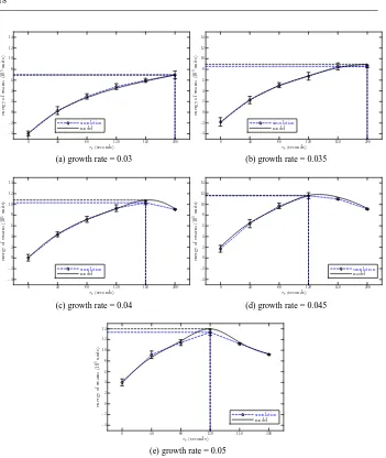
Plotting the relationship between total net energy of the swarm (after 20000 seconds) and the resting time threshold parameterτr of individual robots, Figure 8 compares the results
from the simulation and the model. As we can see, for the same resting time threshold parameter, increasing the growth rate Pnew, increases the total net energy of the swarm.
−4 −2 0 2 4 6 8 10 12 14 en er gy of sw ar m (1 0 5u n it s)
0 40 80 120 160 200
τr(seconds) simulation
model
(a) growth rate = 0.03
−4 −2 0 2 4 6 8 10 12 14 en er gy of sw ar m (1 0 5u n it s)
0 40 80 120 160 200
τr(seconds) simulation
model
(b) growth rate = 0.035
−4 −2 0 2 4 6 8 10 12 14 en er gy of sw ar m (1 0 5u n it s)
0 40 80 120 160 200
τr(seconds) simulation
model
(c) growth rate = 0.04
−4 −2 0 2 4 6 8 10 12 14 en er gy of sw ar m (1 0 5u n it s)
0 40 80 120 160 200
τr(seconds)
simulation
model
(d) growth rate = 0.045
−4 −2 0 2 4 6 8 10 12 14 en er gy of sw ar m (1 0 5u n it s)
0 40 80 120 160 200
τr(seconds)
simulation
model
[image:18.595.74.425.71.487.2](e) growth rate = 0.05
Fig. 8: Comparison of simulated and modelled total net energy of the swarm after 20000 seconds for a swarm of 8 robots with varying resting time threshold parameter. The maximal net energy and the corresponding τr are highlighted with horizontal and vertical dashed
lines.
collect. For the same growth rate, when the rate is below 0.04, the total net energy of the swarm increases withτr increasing. However, for the other three situations the total net
energy doesn’t increase monotonically withτr increasing. It reaches a maximal value and
then falls, i.e. there is an optimal value ofτr in order to achieve maximum net energy for
the swarm. Moreover, the maximal total net energy and the corresponding critical value ofτrvary with Pnewchanging, as shown in Figure 8:(c)(d)(e). Figure 8 illustrates excellent
rates, thus demonstrating that it is more convenient to use the macroscopic probabilistic model to find the optimal value ofτrthan by trial and error with simulation.
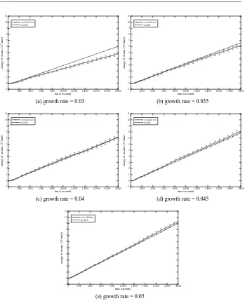
4.1.3 case 3: Pnewnonzero, with adaptation
The third set of experiments are designed to validate the model with the full adaptation capability presented in section 2. We choose a set of arbitrarily selected adjustment factors to test the macroscopic model,{α1,α2,β1,β2,γ1,γ2,η}={5,5,10,10,20,40,20}. With the same set of adjustment factors, we have tested the model with different food growth rates. Figure 9 plots the results from both simulation and the macroscopic probabilistic model, in which the growth rate is varied from 0.03 to 0.05. The error bars represent the standard deviations of data recorded from 10 simulation trials. We see that simulation results fit well to the curves obtained from the macroscopic model, though noting a relatively large gap when the growth rate is set to 0.03 (Figure 9(a)).
4.2 Optimisation of the adaptation algorithm using the genetic algorithm
The challenge we face in optimising the adaptation algorithm is the large solution space for the adjustment factors. These adjustment factors are believed to be correlated with each other, but the relationships between them remain unknown. The simulation of collective foraging using the Stage simulator, running on a 2.6 GHz CPU desktop PC, has a relatively low acceleration ratio over real time. For example, the simulation of a swarm of 8 robots can only achieve an acceleration ratio of about 20, and this value will drop quickly if the swarm size is increased. Since there are no obvious guidelines for manually tuning the parameters of the adaptation algorithm, it is clearly not practical to cover the whole solution space with simulation and a trial and error approach. Given that we have a macroscopic probabilistic model that captures the dynamics of the swarm with reasonable accuracy, the selection of optimal parameters for the adaptation algorithm becomes a multi-parameter optimisation problem with the model in the loop. The objective function can be directly defined as the net energy of the swarm. For each evaluation we need to run the model with the candidate parameters. Although running the model numerically is much faster than the simulation and is not sensitive to swarm size (about 12000 times faster than real time on the same computer), a brute force approach would still be impractical. To reduce the search space to a reasonable size certain constraints must be applied to these parameters. Let us assume all adjustment factors are chosen from a series of bounded positive integer values. Let X= [α1,α2,β1,β2,γ1,γ2,η]represent the solution of the optimisation problem, then a search spaceZfor X can be then defined as
Z={X∈Z7|α1min≤α1≤α1max,α2min≤α2≤α2max, . . . ,ηmin≤η≤ηmax} (40)
Any appropriate search technique can be used to find an approximate optimal solution for the adaptation algorithm. Clearly, the genetic algorithm (GA) is a good candidate.
−1 0 1 2 3 4 5 6 7 8 9 10 11 en er g y o f sw ar m ( 10 5 u n it s)
0 2000 4000 6000 8000 10000 12000 14000 16000 18000 20000
time (seconds)
simulation model
(a) growth rate = 0.03
−1 0 1 2 3 4 5 6 7 8 9 10 11 en er g y o f sw ar m ( 10 5 u n it s)
0 2000 4000 6000 8000 10000 12000 14000 16000 18000 20000
time (seconds)
simulation model
(b) growth rate = 0.035
−1 0 1 2 3 4 5 6 7 8 9 10 11 en er g y o f sw ar m ( 10 5u n it s)
0 2000 4000 6000 8000 10000 12000 14000 16000 18000 20000
time (seconds)
simulation model
(c) growth rate = 0.04
−1 0 1 2 3 4 5 6 7 8 9 10 11 en er g y o f sw ar m ( 10 5u n it s)
0 2000 4000 6000 8000 10000 12000 14000 16000 18000 20000
time (seconds)
simulation model
(d) growth rate = 0.045
−1 0 1 2 3 4 5 6 7 8 9 10 11 en er g y o f sw ar m ( 10 5 u n it s)
0 2000 4000 6000 8000 10000 12000 14000 16000 18000 20000
time (seconds)
simulation model
[image:20.595.74.423.78.507.2](e) growth rate = 0.05
Fig. 9: Comparison of simulated and modelled instantaneous energy of the swarm with adaptive foraging.
generation. Therefore, after some generations, the individuals in the population might all be near-optimal solutions to the original problem.
4.2.1 Rough estimation of the ideal optimal performance
As the best performance of the swarm with adaptation is hard to determine exactly, in or-der to assess the performance of the proposed steady-state GA, we need to estimate the ‘ideal’ optimal performance of the swarm for given environmental conditions (food den-sity). Clearly, to obtain the maximal net energy, the swarm needs to collect as much energy as possible whilst keeping energy consumption as low as possible. For a growth rate Pnew,
Pnew×Tdur food-items grow during a period Tdur. Since – ideally – all of them would be
collected during this period, then the total energy retrieved by the robots is
Eretrieval=EcPnewTdur (41)
The minimum energy consumed by the swarm with N0robots can be expressed as
Econsumed=EsPnewTdurTret+Er(N0Tdur−PnewTdurTret) (42)
The first term in the RHS of Equation(42) represents the energy consumed by the robots in order to collect all food-items. The second term represents the energy consumed by the robots resting in the nest. Tret is the minimal average time for a successful retrieval, which
can be expressed as the sum of Tgand Td. Thus, the ideal optimal net energy that the swarm
can achieve is expressed as follows.
Enet=EcPnewTdur−(Es−Er)PnewTdur(Tg+Td)−ErN0Tdur (43)
4.2.2 Optimal performance
Next we run the steady-state GA to optimise parameter selection under different environ-mental conditions. We set the population size to 30 individuals and, in each generation of the GA, the worst half will be replaced. The GA records the scores of the best-of-generation individuals for the most recent 30 best-of-generations. The termination condition is that
Table 3: Constraints for the adjustment factors.
parameters α1 α2 β1 β2 γ1 γ2 η
min 0 0 0 0 0 0 0
max 64 64 100 100 100 100 100
interval 2 2 5 5 5 5 5
the same best-of-generation individual repeats in the last 30 generations. Table 3 gives the constraints applied to the search space. Adjustment factors are now selected from interval-based sets. For example,α1 could be 0,2,4,6, . . .64. The boundary for each parameter is
selected intuitively. To evaluate the fitness of each chromosome, the macroscopic model is run with Tdur =20000 seconds. Different environmental conditions are considered by
choosing Pnew=0.040 or Pnew=0.045. Three cases are chosen to test the GA:
case 1: Pnew=0.040, both Trand Tsare adjustable;
0.5 0.6 0.7 0.8 0.9 1 1.1
fi
tn
es
s
(1
0
6)
0 10 20 30 40 50 60 generation
(a) case 1
0.5 0.6 0.7 0.8 0.9 1 1.1 1.2 1.3
fi
tn
es
s
(1
0
6)
0 10 20 30 40 50 60 70 80 90 generation
(b) case 2
0.5 0.6 0.7 0.8 0.9 1 1.1 1.2 1.3
fi
tn
es
s
(1
0
6)
0 10 20 30 40 50 60 generation
[image:22.595.73.421.79.361.2](c) case 3
[image:22.595.81.410.427.478.2]Fig. 10: Convergence of average fitness of the population, population size is 30.
Table 4: Best set of adjustment factors found by the GA and the corresponding net energy of the swarm.
case Pnew α1 α2 β1 β2 γ1 γ2 η predicted net energysimulation ideal
1 0.040 0 16 0 0 50 65 30 1077469 1057594 1180800
2 0.045 2 16 5 0 65 20 5 1261147 1195620 1348400
3 0.045 0 0 0 5 0 85 0 1221298 1150095 1348400
case 3: Pnew=0.045, Tris adjustable, but Tsis fixed.
Figure 10 plots the evolution of average fitness of the population for these three cases. The rapid improvement in the average fitness can clearly be seen in the first few generations in Figure 10. The corresponding best-of-generations are shown in Table 4. As the chromo-some in the GA is mapped directly to the solution space for the adaptation algorithm, Table 4 gives also the net energy of the swarm obtained from the macroscopic model (predicted), the simulation, and Equation (43) (ideal). For each case, the predicted net energy of the swarm has reached over 90% of the ideal values (91.2%, 93.5% and 90.6% respectively). Given that 1) Tret is roughly estimated 2) no failure retrievals are taken into account 3) we
assume all the food-items are collected during Tdurand 4) no interference between robots is
We also see in Table 4 that, although there is no adaptation of searching time threshold in case 3, the swarm can still achieve near-optimal performance with a certain combination of adjustment factors, obtained from the GA. This implies that the searching time threshold has less effect on the performance of the swarm than the resting time threshold. Consider the roles of these two time threshold parameters: the resting time threshold determines how long the robots have to rest in the nest, with a direct effect on the energy of the swarm; while the searching time threshold only has an effect when robots take too long searching in a relatively low food density environment. In most cases, however, the robots succeed in finding food before their searching time expires. Thus, adaptation of the resting time threshold parameter is more important than adaptation of searching time threshold.
5 Conclusions
This paper has described a macroscopic probabilistic model developed to investigate the ef-fect of individual parameters on the group performance, and hence optimise the controller design, for a swarm of robots engaged in collective adaptive foraging for energy. A prob-abilistic finite state machine has been presented, and a set of difference equations derived, to describe collective foraging at the macroscopic level. The first challenge in modelling adaptive collective foraging is that of dealing with nested time parameters and their dif-ferent priorities. Although it is fairly straightforward to write down most of the difference equations for the proposed PFSM, deriving a mathematical description which captures the changes in number of unsuccessful robots (i.e. that failed to find food), as a function of searching time threshold, is challenging. We have achieved this by introducing the idea of a time-limited sub-PFSM into the model. This sub-PFSM evolves with the full PFSM but represents only the sub-set of robots engaged in the so-called “searching-grabbing” task.
As macroscopic probabilistic modelling approaches are built upon the theory of stochas-tic processes, they do not take the exact trajectory of individual robots into account. It is therefore difficult to deal with the heterogeneities in the swarm due to the differences in control parameters. With adaptation, the resting time and searching time thresholds are dif-ferent from robot to robot, even from one time step to the next. The second challenge is, therefore, that of how to build these differences into the macroscopic model. To solve this problem, in conjunction with the idea of the sub-PFSM, we have introduced private resting and searching time thresholds, and their counterparts – public resting and searching time thresholds. The private time thresholds are valid for a sub-set of robots within the sub-PFSM and play the role of deciding when the transition from one state to another is triggered, while the public time thresholds are used to link all of the private time parameters created each time step; they affect each other in a bi-directional manner. The adaptation rules are then modelled by adjusting the private/public time threshold parameters accordingly.
we have tested the near-optimal solutions in simulation trials, and results again show that there is good quantitative agreement with the macroscopic probabilistic model.
We have also shown that our macroscopic model of adaptive foraging can be used to investigate the efficiency of the system, in terms of swarm size, in the standard robot foraging task, similar to that presented in Lerman (2002). But compared with Lerman’s model, our downgraded model (with pnew=0, and no adaption) represents the foraging task with more
detailed behaviours, in particular competition between robots, and with no free parameters at all. This is one of the reasons the full model is presented in a fairly complex form. However, the complexity of the model lies mainly in the challenges of modelling the adaptivity of the system from individual robot level to group level; to the best of our knowledge this has not been fully investigated to date. Our model has aimed to represent the adaption rules for the individual robot while minimising complexity. Indeed, we would argue that our PFSM model is as simple as it can be given the purpose of the model, i.e. as a tool to analyse and hence optimise the design of the adaptation rules of the swarm system. We also note that mean-field approaches such as the proposed macroscopic model do not capture the randomness of the system. If that is the main interest of the modelling effort a microscopic probabilistic approach, as introduced by Martinoli et al (1999), should be applied. However, given the complexity of the adaptation rules a microscopic model of adaptive foraging – even if it could be constructed – would also have high complexity.
In conclusion, we have demonstrated that the macroscopic probabilistic modelling ap-proach can be successfully extended to model the heterogeneities of the swarm using sub-PFSMs and averaging techniques. The sub-PFSM solves the nested dynamics problem of the two nested time parameters, and provides a way to model the differences between indi-viduals at a macroscopic level. Although the techniques presented in this paper have been developed to model adaptive foraging, the structure of the PFSM presented for this case study is not atypical, thus we argue that these techniques are generally applicable to the class of heterogeneous (in control parameters) swarm systems with similar dynamics. In swarm robotics macroscopic modelling provides us with a powerful tool for gaining a deeper un-derstanding of the effect of individual robot characteristics on the overall performance of the collective, and therefore guiding performance optimisation of the individual robot con-trollers.
Acknowledgments
This work was partially supported by the EU Asia-link Selection Training and Assessment of Future Faculty (STAFF) project. We are also indebted to the anonymous reviewers for the many insightful comments which have guided the improvement of this paper.
Appendix: Estimation of transition probabilities and time parameters
Transition probabilitiesγf,γr,γl, and time parameters Tg, Th, Td, can be obtained analytically
by considering robot control strategies together with the following three assumptions:
– food-items are uniformly dispersed in the arena, over time;