3 4 5 6 7 8 9 10 11 12 13 14 15 16 17 18 19 20 21 22 23 24 25 26 27 28 29 30 31 32 33 34 35 36 37 38 39 40 41 42 43 44 45 46 47 48 49 50 51 52 53 54 55 56 57 58 59 60 61
Short term electricity demand forecasting using partially linear
additive quantile regression with an application to the unit
commitment problem
∗
Moshoko Emily Lebotsa1, Caston Sigauke∗1, Alphonce Bere1, Robert Fildes2, John E Boylan2
1Department of Statistics, University of Venda, Private Bag X5050
Thohoyandou, 0950, South Africa
2Lancaster Centre for Marketing Analytics and Forecasting, Department of Management Science
University of Lancaster, United Kingdom
March 28, 2018
Abstract
Short term probabilistic load forecasting is essential for any power generating utility. This paper discusses an application of partially linear additive quantile regression models for predicting short term electricity demand during the peak demand hours (i.e. from 18:00 to 20:00) using South African data for January 2009 to June 2012. Additionally the bounded variable mixed integer linear programming technique is used on the forecasts obtained in order to find an optimal number of units to commit (switch on or off. Variable selection is done using the least absolute shrinkage and selection operator. Results from the unit commitment problem show that it is very costly to use gas fired generating units. These were not selected as part of the optimal solution. It is shown that the optimal solutions based on median forecasts (Q0.5 quantile forecasts) are the same as
those from the 99thquantile forecasts except for generating unitg8c, which is a coal fired unit. This shows that for any increase in demand above the median quantile forecasts it will be economical to increase the generation of electricity from generating unit g8c. The main contribution of this study is in the use of nonlinear trend variables and the combining of forecasting with the unit commitment problem. The study should be useful to system operators in power utility companies in the unit commitment scheduling and dispatching of electricity at a minimal cost particularly during the peak period when the grid is constrained due to increased demand for electricity.
Keywords: Lasso, mixed integer linear programming, quantile regression, short term peak load forecasting, unit commitment.
1
Introduction
1.1 Context
6 7 8 9 10 11 12 13 14 15 16 17 18 19 20 21 22 23 24 25 26 27 28 29 30 31 32 33 34 35 36 37 38 39 40 41 42 43 44 45 46 47 48 49 50 51 52 53 54 55 56 57 58 59 60 61 62 63 64
balance [34]. Load forecasts are also required for many other purposes such as system security, rate design, revenue projection as well as for scheduling activities [19,20,47]. Moreover, load forecasts are usually assessed periodically, ranging from hours, days, and weeks, months, up to a year, or even longer. However, the focus in this paper is on the short term load forecasts (STLF) which range from few hours up to a week [1]. Accurate and efficient forecasts are necessary for any power supplying company as they help in preventing problems such as under loading (i.e. load shedding, blackouts, etc.) or overloading (i.e. producing more capacity than needed), which are very costly to suppliers [34]. Accurate forecasts also help with the unit commitment decisions by reducing production costs [2].
1.2 An overview of the literature on load forecasting
Short term load forecasting (STLF) has been receiving a lot of attention [10]. Almost every year
different models for STLF are developed, applied, reviewed and published. Short term forecasts
are used to estimate the load demand up to a week ahead of a schedule [16]. Many utilities rely on them because they are useful when it comes to daily operation and scheduling of power systems
[31]. For instance, obtained forecasts are used to schedule generation as well as transmission of
units to consumers. A brief review on weather station and variable selection methods together with other methods used in short term forecasting as well as on the unit commitment problem (UC) follows.
South Africa (SA) is among developing countries around the world faced with electricity crisis. On the African continent, SA is considered as the most industrialized country with the highest electricity consumption [33]. The electricity demand pattern is complex in nature, due to the presence of several factors such as the economic, environmental, weather conditions and calendar effects [9,10]. However, many researchers use temperature in their forecasting models as it is one of the major drivers of electricity demand. A South African study that uses temperature is that of Chikobvu and Sigauke [5], their main aim being to assess its impact on the daily peak electricity demand. The results show that electricity demand is sensitive to cold weather in the country. Another study that examines meteorological effects is that of Taylor and MacSharry [42], in which the seasonality patterns and their effects were studied from European countries.
Other than meteorological effects, time factors also have a huge impact on electricity demand. Time factors include day-of-week, yearly seasonality, time of the day, etc. and generally are known as calendar effects and their impact in short term load forecasting are discussed in detail by [9]. For instance, load curves were used to explain electricity consumption patterns for different hours during the day and based on the load curves these two authors concluded that calendar effects mostly determine the daily life style of the consumers, i.e. highest peak load in the evening [9]. Moreover, the peak load demand is the most studied as highlighted by Hinman and Hickey [19].
6 7 8 9 10 11 12 13 14 15 16 17 18 19 20 21 22 23 24 25 26 27 28 29 30 31 32 33 34 35 36 37 38 39 40 41 42 43 44 45 46 47 48 49 50 51 52 53 54 55 56 57 58 59 60 61
Another important aspect in model building is to be able to identify the best set of input variables. For instance, over the past years many different variable selection methods have been used to select important variables to include when forecasting generally. There are many different available methods that can be used to select important variables in a study. These include the dimension reduction, shrinkage as well as the subset selection methods [27]. The most commonly used methods are subset selection which include techniques such as the stepwise criterion and many more.
A study that applied one of the variable selection methods mentioned above is that of Fan and Hyndman [10]. The authors in this paper used a stepwise variable selection technique was used to select a combination set of variables that were then used in models that were used to predict 48 half-hourly load demand in Australia. The authors used the stepwise backward selection method which involves including all the variables at first and removing one at a time while keeping the rest in the model. Then they continued by checking the performance of the model with removed variable using mean absolute percentage error (MAPE). Thus if the model resulted with a lower MAPE value, it was then selected as the best model for that period.
Although stepwise variable selection methods have been and are still widely used, they have
limitations. Some of these limitations include their inability to deal with multicollinearity and
less computational efficiency. These limitations are mostly ignored in many studies. For instance,
according to Olusegun et al. [35] the stepwise selection criterion selects variables based on the
correlation between a response and a set of explanatory variables only. Somehow the correlation within the explanatory variables is not considered which can lead to having one or more variables with the same characteristics in the model, due to their multicollinearity. Shrinkage methods are better equipped to handle multicollinearity.
Several methods have been proposed in the literature on variable selection in regression based models. In this study we use least absolute shrinkage and selection operator (Lasso) via hierarchical interactions. For modelling time series data with multiple seasonalities Bien et al. [3] developed a Lasso for hierarchical pairwise interactions in regression based models. In another study a method which satisfies the strong hierarchy for learning linear interaction models is presented in [32]. Results show that the developed method is comparable with past methods. The method caters for both continuous and categorical variables.
6 7 8 9 10 11 12 13 14 15 16 17 18 19 20 21 22 23 24 25 26 27 28 29 30 31 32 33 34 35 36 37 38 39 40 41 42 43 44 45 46 47 48 49 50 51 52 53 54 55 56 57 58 59 60 61 62 63 64
On the other hand, quantile regression (QR) models are used a lot in forecasting by different energy sectors, e.g. wind power forecasting, price forecasting, etc. A recent study [14], introduced an optimal forecast quantile regression (OFQR) model which was used to forecast the annual peak electricity demand in 32 zones in United States (US). The main aim was to compare the relative performance of the OFQR model with the ordinary least square (OLS) regression model, which is a standard method used by almost every utility. The OFQR model provided more accurate forecasts compared to OLS.
In another study, a QR model was also used to forecast electricity demand [41]. The data used in their study was collected from 3639 households in Ireland at both aggregated and disaggregated
levels. The proposed QR model was compared with three other benchmark methods. Other
authors also developed additive quantile regression models for forecasting both probabilistic load and electricity prices as part of the global energy forecasting competition of 2014 (GEFCom2014)
[13]. A summary of the methods used in GEFCom2014 are given in [20]. The proposed new
methodology of [13] ranked first in both tracks of the competition. The work done by [13] is
extended by Fasiolo et al. [11] who developed fast calibrated additive quantile regression models.
To implement the developed models, [11] developed a new r statistical package “qgam”. The same
covariates used in [13] were also used in [11]. In both papers variable selection techniques are not discussed. In another study [18] used kernel support vector quantile regression and copula theory
for short-term load probability density forecasting. Two criteria for evaluating the accuracy of
the prediction intervals are proposed, the prediction interval normalized average width (PINAW) and the prediction interval coverage probability (PICP). Results from this study show that the Gaussian kernel gives the most accurate forecasts compared to the linear and polynomial kernels respectively. In a more recent study, [48] developed a Gaussian process quantile regression model for short-term load probability density forecasting. The authors argue that this modelling framework provides accurate point forecasts as well as giving probabilistic descriptions of the prediction intervals.
The present study discusses an application of partially linear additive quantile regression (PLAQR) models in forecasting hourly electricity demand during the peak period (i.e from 18:00 to 20:00) in South Africa (SA). PLAQR models are a combination of generalized additive models (GAMs) developed by [17] and quantile regression (QR) models [29,30] where the conditional quantile function
comprises a linear parametric component and a nonparametric additive component [23]. Among
the first to introduce partially linear models include among others Engle et al. [8] who analyzed the relationship between electricity usage and temperature. A two-step approach for estimating a PLAQR model is discussed in Hoshino [23] and applied to a real data set. In a another study [28] discussed an application of double-penalized quantile regression partially linear additive models. A simulation study and an application to a real data set were used to evaluate the developed models. In a related study, Bayesian partially linear additive quantile regression models are used in simulation studies by [24]. To summarize, the state-of-the-art in modelling is to use hybrid models.
1.3 Literature review on the unit commitment problem
6 7 8 9 10 11 12 13 14 15 16 17 18 19 20 21 22 23 24 25 26 27 28 29 30 31 32 33 34 35 36 37 38 39 40 41 42 43 44 45 46 47 48 49 50 51 52 53 54 55 56 57 58 59 60 61
quirements [45]. Such an application is useful as it helps prevent losses and minimize fuel consumption.
In a study by Kurban and Filik [31], a method that combined short term load forecasting with UC in order to reduce production costs in one of the thermal plants based in Kutahya region, Turkey was proposed. The authors proposed two models which were used to forecast electricity demand and then used the forecasts obtained to find solutions to a UC problem using the Lagrange relaxation method. The empirical results indicated that accurate load forecasting is essential for UC.
In another study considered the stochastic model for the long term solution on security-constrained unit commitment (SCUC) problem is that of Wu et al. [46]. SCUC is an “extension of the basic UC problem that includes additional factors such as fuel, emission and transmission constraints” [45]. These factors were not included in the early stochastic problems (SP) [6]. The proposed model was used to capture the uncertainties of generation components (i.e. generation units and transmission lines) as well as the inaccuracy of the load forecasts.
In order to meet forecast demand it is important to plan in advance the start-up and shut down schedules of power generating units. This has to be done in an optimal way so as to minimize total generation and start-up costs while ensuring that load demand and reserve margin requirements are met. This calls for probabilistic load forecasts which help system operators in planning the scheduling of generating units. A review that surveys the latest optimization methods to solve the UC problem in deterministic and stochastic cases is presented in Saravanan et al. [38]. The paper presented the planning of the running time for different production units so as to meet the constraints under various scenarios. But the authors underlined the fact that it is very difficult to meet all of the constraints in one optimization technique. They also categorized the optimization methods into conventional
and non-conventional ones. They focused on the novel hybrid algorithms through classical and
non-classical methods. Finally, the authors tabulated UC papers for the last decade, in the interest of new researchers in the field, and briefly discussed a variety of techniques such as hybrid Lagrangian relaxation, particle swarm optimization (PSO) and hybrid genetic algorithms.
A review of past and present findings was done in order to provide a detailed understanding of the UC [45]. The UC aims at scheduling the most cost-effective association of electricity production from a couple of units, during a specific period of time, under some units and transmission restrictions [45]. The author underlined that the UC is a large-scale sequential problem often involving a large number of generating units, making it difficult to obtain, in a reasonable period of time, an optimal solution. The paper affirmed that on the US markets, the most used, among several optimization techniques, are mixed integer linear programming (MILP) and Lagrangian relaxation (LR). The two approaches are briefly discussed and compared in the paper. The author concluded in admitting that the UC problem is far from fully solved, and many researchers preferred new hybrid techniques that combine different optimization techniques. An open software components used in short-term load forecasting combined with the unit commitment problem was presented by Short et al. [40]. The empirical results showed a reduction in costs and improved efficiency as a result of balancing market interactions in the presence of prediction inaccuracies in the proposed modelling framework.
1.4 Contributions
6 7 8 9 10 11 12 13 14 15 16 17 18 19 20 21 22 23 24 25 26 27 28 29 30 31 32 33 34 35 36 37 38 39 40 41 42 43 44 45 46 47 48 49 50 51 52 53 54 55 56 57 58 59 60 61 62 63 64
improves the forecast accuracy. Secondly weather stations in this study are selected based on cluster analysis. They were selected in such a way that they represent the different parts of South Africa (SA). For each cluster, the data were aggregated to get the maximum, minimum and average daily temperature. Coastal and inland temperature data were also used as separate variables in the models. The analysis was done on the overall aggregated as well on the non-aggregated temperature data set. The third contribution involves the use of the bounded variable mixed integer linear programming (BVMILP) in solving the unit commitment problem during the peak period.
2
Models
Partially linear additive quantile regression (PLAQR) models including variable selection and estima-tion of parameters are discussed in this secestima-tion.
2.1 Partially linear additive quantile regression models
Generalized additive models (GAMs) which allow flexibility in modelling of predictors as a sum of smooth functions were developed by [17]. Quantile regression (QR) on the other hand was developed by [29] as a modelling framework for estimating the conditional median, including the full range of other conditional quantiles. The partially linear additive quantile regression models are a combination of GAMs and QR models. A PLAQR model is given in Eq. (1) [23]:
yth=β0h,τ + p1
X
j=1
sjh,τ(xthj) + p2
X
j=1
βhj,τzthj+εth,τ, τ ∈(0,1) (1)
whereyth, t= 1, ..., nis the response variable which is electricity demand on daytat hourh,p=p1+p2
is the total number of input variables which includes linear and non linear variables,h= 1, ...,24,xthj
are continuous variables,sjh,τ are smooth functions,zthj are linear variables,βhj,τ are parameters and
εth,τ is the quantile error term. Eq. (1) can be written in matrix form as:
Y=sτ(X) +ZTβτ+ετ, τ ∈(0,1). (2)
Let Y =F(X,Z, τ) then τ =P(Y ≤F(X,Z, τ). The parameter estimates of Eq. (2) are obtained
by minimizing the following function
QY|X,Z(τ) = n X
i=1
ρτ Yi−ZiTβ−s(X)
, (3)
whereρτ(u) ={τI(u≥0) + (1−τ)I(u <0)} |u|={τ−I(u <0)}u is the quantile loss function.
Since the residuals, εth,τ of the hourly load models are autocorrelated it is important that the
auto-correlation is significantly reduced before the models are used for forecasting. In this study we use the following procedure in modelling residual autocorrelation.
1. We estimate the parameters in Eq. (3) and extract residuals, εth. An appropriate
SARIMA(p,d,q)× (P,D,Q)[s] is then fitted,
2. The fitted values of the residuals of the SARIMA(p,d,q) × (P,D,Q)[s] are subtracted from yth
to getyth∗ and we then regressyth∗ on the covariates,
3. The residual autocorrelation in the new model is then checked. If the residuals are still autocor-related the process is repeated until the desired results of uncorautocor-related errors are achieved.
6 7 8 9 10 11 12 13 14 15 16 17 18 19 20 21 22 23 24 25 26 27 28 29 30 31 32 33 34 35 36 37 38 39 40 41 42 43 44 45 46 47 48 49 50 51 52 53 54 55 56 57 58 59 60 61
2.2 Data and variables
Let yth denote electricity demand (measured in MegaWatts (MW)) on day t at hour h, where
t = 1, ..., n and h = 1, ...,24 with the corresponding covariates xth1, xth2, ..., xthp as discussed in
Section 2.1. In this study the following hours (hrs) are considered 18:00, 19:00 and 20:00, i.e.
h =18:00, 19:00 and 20:00. Daily load profiles in South Africa show that it is during this period
that peak demand is experienced [39, among others]. The variables used in this study are the load at 18:00, 19:00 and 20:00 hrs which is used as the response variable and the predictor variables are calendar effects, temperature and lagged demand. Lag1 and Lag2 simultaneously represent the lagged electricity demand for the same hour of the first and second previous days. Both the lags are differenced in order to make the series of the electricity demand stationary. According to [10] the inclusion of lagged demand effects reduce autocorrelation, however it does not completely remove it. DPED, AED were used to represent daily peak electricity demand and the average electricity demand for the past 24 hours.
The calendar variables considered in this study are denoted as Daytype, DBH, DH, DAH, representing the day of the week, the day before a holiday, day holiday, day after holiday respectively. Daytype is coded as 1 for Monday, 2 for Tuesday up to 7 for Sunday while the variable month is coded as 1 for January, 2 for February up to 12 for December. The variables DBH, DH and DAH were coded as follows, DBH takes value 1 if it is a day before a holiday and 0 otherwise, and similarly DH takes value 1 if the day is a holiday and 0 otherwise and DAH takes value 1 if its a day after a holiday and 0 elsewhere. Hourly temperature data used in this paper is from 28 South African weather stations. Initially all the weather stations in the country were considered and those which were selected for the study were in such a way that they represent the whole country. For the purposes of this study the selected stations were split into two main thermal regions, i.e. coastal and inland. This means that the aggregated coastal and inland temperature variables are considered in this paper including the overall aggregated temperature for the whole country which are are used for comparison sake.
The temperature variables are average daily coastal temperature (ADTC), average maximum and minimum coastal temperature (maxTC and minTC), average minimum, average maximum, average daily inland temperature (minTI, maxTI and ADTI), average minimum of coastal and inland tem-peratures (AminTCI), average of average daily coastal and inland temtem-peratures (AADTCI), average maximum of coastal and inland temperatures (AmaxTCI), difference between average minimum of coastal and inland temperatures (DminTCI), difference between average maximum of coastal and inland temperatures (DmaxTCI), difference between average of average daily coastal and inland tem-peratures (DADTCI). A nonlinear trend variable (noltrend) is also used as a covariate. This trend variable is determined by fitting a penalized cubic smoothing spline to the response variable. The fitted values are then extracted and used for the nonlinear trend variable. The data is for the period January 2009 to June 2012. The data for the period January 2009 to December 2011 is used for training, while the remaining data i.e. January to June 2012 used for testing.
2.3 Variable selection, parameter estimation and forecast combination
2.3.1 Variable selection
6 7 8 9 10 11 12 13 14 15 16 17 18 19 20 21 22 23 24 25 26 27 28 29 30 31 32 33 34 35 36 37 38 39 40 41 42 43 44 45 46 47 48 49 50 51 52 53 54 55 56 57 58 59 60 61 62 63 64
Letythbe electricity demand as defined in Eq. (1), with corresponding covariateszth1, ..., zthpin which
pairwise interactions are allowed between the predictors. In this study quadratic interactions are not
allowed, i.e. zthi×zthk wherei=k. The model is given as [3]:
yth = β0h,τ + X
i
βhi,τzthi+ X
i6=k
αikzthizthk+εth,τ. (4)
The Lagrangean form of the strong hierarchical Lasso is ([3]):
min
β0∈R,β∈Rp,α∈Rp×p,α=αT
h(β0, β, α) +λ X
i
max{|βi|,kαikk1}+
λ
2kαk1 (5)
whereh(β0, β, α) is a quadratic loss function given as
h(β0, β, α) =
1 2
n X
t=1
yth−β0h−zthTβh− 1
2z
T thαzth
!2
(6)
Whilst Eq. (4) shows interactions for linear variables, it should be noted that the interactions can be applied to nonlinear variables as well.
2.3.2 Parameter estimation
An adaptation of the Barrodale and Roberts algorithm for`1−regression will be used to estimate the
PLAQR model parameters. The simplex approach to solving the general`1-regression problem [30,36]
is given as follows:
minβ∈Rp
n X
i=1
ρτ Yi−ZiTβ−s(X)
(7)
This is then reformulated as a linear programming problem. Two artificial variables,ui, vi, i= 1, ..., n
are introduced to represent the positive and negative parts of the vector of residuals. This results in a new problem.
minβ,u,v∈R×R2n
+
1Tu+1Tv|y=Zβ+u−v,(u, v)∈R2+n , (8)
where1 is a vector of ones. The dual formulation of Eq. (8) is
max
yTα|Zα= 0, α∈[−1,1]n (9)
and settingb=α+121results in
max
yTb|Zb= 1
2Z
T1, b∈[0,1)n
. (10)
2.3.3 Forecast combination
Combining forecasts improves the forecast accuracy [7,13, among others]. Let K denote the number
of methods used to forecast the response variable, then the combined forecasts will be calculated as follows:
fth= K X
k=1
ωkthykth (11)
where ωkth is the weight. The pinball loss function is used as an evaluation criterion. In this study,
6 7 8 9 10 11 12 13 14 15 16 17 18 19 20 21 22 23 24 25 26 27 28 29 30 31 32 33 34 35 36 37 38 39 40 41 42 43 44 45 46 47 48 49 50 51 52 53 54 55 56 57 58 59 60 61
2.4 Error measures for probabilistic forecasting and evaluation of methods
Scoring rules are used to assess and compare the probabilistic models in this study. A scoring rule
assigns a penalty score S(y, F) where y is the observation used for forecast evaluation and F is the
forecast distribution [15]. A smaller score corresponds to a better forecast. This study uses three of the commonly used error measures in probabilistic forecasting which are the continuous rank probability score (CRPS), logarithmic score (LogS) and the quantile loss function also known as the pinball loss function.
2.4.1 Continuous rank probability score
The CRPS measures the distance between the predicted and the observed cumulative density functions (CDFs) of scalar variables [15].
CRPS(y, F) =
Z 1
0
QSτ F−1(τ), ydτ (12)
whereF is the forecast distribution and QSτ is the quantile score given as:
QSτ F−1(τ), y= 2 Iy≤F−1(τ)−τ F−1(τ)−y (13)
2.4.2 Logarithmic score
The logarithmic score (LogS), is given by
LogS(y, F) =−logf(y) (14)
wheref is the density function for the forecast distribution.
2.4.3 Quantile loss function
The quantile loss function also known as the pinball loss function is given by:
L( ˆQY|X,Z(τ)) = (
τ(y−QˆY|X,Z(τ)) ify≥QˆY|X,Z(τ) (1−τ)( ˆQY|X,Z(τ)−y) ify <QˆY|X,Z(τ)
(15)
where ˆQY|X,Z(τ) is the quantile forecast and y is the observation used for forecast evaluation.
2.4.4 Skill score (improvement rate)
The performance of the methods against the best methods for each of the peak hours is calculated using Eq. (16)
Improvement(%) =
1− Pinball(best method)
Pinball(other method)
×100 (16)
6 7 8 9 10 11 12 13 14 15 16 17 18 19 20 21 22 23 24 25 26 27 28 29 30 31 32 33 34 35 36 37 38 39 40 41 42 43 44 45 46 47 48 49 50 51 52 53 54 55 56 57 58 59 60 61 62 63 64
2.5 Unit commitment
In this study the bounded variable mixed integer linear programming (BVMILP) method is used in solving the unit commitment problem. The BVMILP is a special class of linear programming technique where some of the variables are restricted to integer values but the rest are ordinary continuous variables and all variables are bounded. The present study intends to demonstrate how the forecasts can be used in solving the UC problem.
Let PGiht be load from generating unit i, i = 1, ..., m at hour h, h =18:00,19:00,20:00 on day t, t =
1, ..., n; PGht national system load at hour h on day t; Pht
Gi(min) the lower limit of the unit power
output;Pht
Gi(max) the upper limit of the unit power output;x
ht
i the 0-1 variable (In this study we will
assume that during the peak period all units are up, i.exhti = 1 for all units);Fsi the start up cost of
unitiat hourh (in this study we will assume that the start up cost is zero);Pht
R the power reserve at
hour h on day t; Fi the average production cost of uniti (cost/MW). In this study we are going to
use fuel cost to represent average production cost per megawatt produced.
Generating units are classified into 13 coal-fired, 1 nuclear, 4 gas, 2 pumped storage and 2 hydroelectric.
These will be denoted as: g1c, g2c, ..., g13c, g14n;g15g, ..., g18g, g19p, g20p, g21h, g22h. As stated by [45], the
main objective of the UC is to minimize cost of generating units over a particular period. Generally, we minimize:
min H X
h=1 m X
i=1 h
Fi
PGiht
xhti +Fsi(ht)xhti i
=F
PGiht, xhti
(17)
The constraints are: Load balance equation
m X
i=1
PGihtxhti =PDht, h= 18,19,20, t= 1, ..., n (18)
Generator power output limits
xhti PGimin ≤PGiht≤xhti PGimax, h= 18,19,20, t= 1, ..., n, i= 1, ..., m (19)
Power reserve constraints
m X
i=1
PGimaxxhti ≥PDht+PRht, h= 18,19,20, t= 1, ..., n (20)
The power reserve constraints ensure that system is reliable and stable. Minimum up/downtime constraints
Uhtup−1,i−Hiup xhti −1−xhti ≥0, h= 18,19,20, t= 1, ..., n, i= 1, ..., m (21)
Uhtdown−1,i−Hidown xhti −xht
−1 i
≥0, h= 18,19,20, t= 1, ..., n, i= 1, ..., m (22)
In this studym= 22.
3
Empirical results and discussion
6 7 8 9 10 11 12 13 14 15 16 17 18 19 20 21 22 23 24 25 26 27 28 29 30 31 32 33 34 35 36 37 38 39 40 41 42 43 44 45 46 47 48 49 50 51 52 53 54 55 56 57 58 59 60 61
3.1 Exploratory data analysis
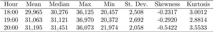
[image:11.612.124.497.239.295.2]The summary statistics for hours considered as the peak period (i.e.18:00, 19:00 and 20:00) in this paper are shown in Table 1. Note that the sampling period considered is from January 2009 to June 2012. For each of the three hours the maximum demand is 36,125MW, 36,970MW and 36,073MW respectively. The skewness and kurtosis presented in Table 1 show that the distributions of the three hours are non-normal. A typical daily load profile over the sampling period is given in Fig. 1 which
Table 1: Summary statistics for electricity demand (MW) at hours 18:00, 19:00 and 20:00.
Hour Mean Median Max Min St. Dev. Skewness Kurtosis
18:00 29,965 30,276 36,125 20,457 2,508 -0.2317 3.0012
19:00 31,063 31,121 36,970 20,372 2,692 -0.2920 2.8814
20:00 31,195 31,451 36,073 21,974 2,058 -0.5422 3.5533
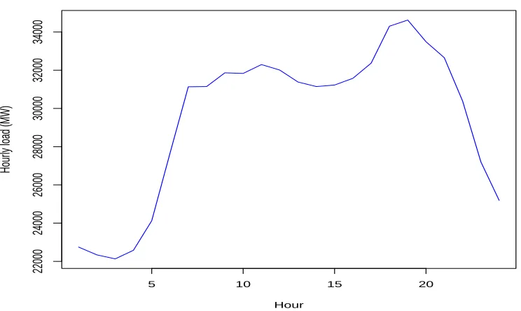
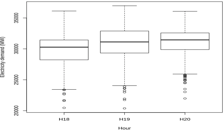
shows that the peak load occurs between 18:00hrs and 20:00hrs. Forecasting electricity demand during this period is very very important to system operators as they have to balance the high demand with what can be supplied by power plants. The highest peak is around 19:00hrs. The South African daily electricity demand time series and density plots for the peak period considered in this paper are as shown in Fig. 2. The panels on the left of Fig. 2 show the time series plots while those on the right panels show the density plots of the demand for 18:00, 19:00 and 20:00 hours respectively. Note that the seasonality patterns of electricity demand in SA on the left panels of Fig. 2, i.e. the plots indicate higher electricity demand in winter and lower demand in summer yearly. The densities on the right panels of Fig. 2 also show that the distributions of the three hours do not follow normal distributions which is consistent with the skewness and kurtosis reported in Table 1. The distributions of electricity demand are further highlighted by the box and whisker plots in Fig. 3.
6 7 8 9 10 11 12 13 14 15 16 17 18 19 20 21 22 23 24 25 26 27 28 29 30 31 32 33 34 35 36 37 38 39 40 41 42 43 44 45 46 47 48 49 50 51 52 53 54 55 56 57 58 59 60 61 62 63 64
Hour
Hour
ly load (MW)
5 10 15 20
22000
24000
26000
28000
30000
32000
[image:12.612.114.486.117.339.2]34000
Figure 1: Typical daily load profile.
3.2 Forecasting results
The PLAQR models with interactions (cross effects) whose variables we got using Lasso via hierarchical interactions are:
yt(18)=β0(18)+ DH+bs(Daytype)+bs(DPED)+bs(AED)+bs(maxTI)+bs(DmaxTCI)+bs(noltrend)
+bs(Lag1)+bs(Lag2)+bs(month)+bs(AED,DmaxTCI)+bs(AED,month) +εt(18)(23)
yt(19)=β0(19)+ DH+bs(Daytype)+bs(DPED)+bs(AED)+bs(maxTI)+bs(minTI)+bs(noltrend)
+bs(Lag1)+bs(Lag2)+bs(month)+bs(maxTI,Lag1)+bs(noltrend,Lag1)+bs(noltrend,Lag2) +εt(19)(24)
yt(20)=β0(20)+ DH+ bs(DPED)+bs(minED)+bs(AED)+bs(maxTC)+bs(minTI)+ bs(noltrend) +bs(Lag1)+bs(Lag2)+bs(month)+bs(DPED,month)+bs(AED,noltrend)+bs(maxTC,Lag2)
+bs(minTI,Lag2)+bs(noltrend,Lag1) +εt(20)(25)
6 7 8 9 10 11 12 13 14 15 16 17 18 19 20 21 22 23 24 25 26 27 28 29 30 31 32 33 34 35 36 37 38 39 40 41 42 43 44 45 46 47 48 49 50 51 52 53 54 55 56 57 58 59 60 61
Demand at 18:00
Year
Demand at 18:00 (MW)
2009.0 2010.0 2011.0 2012.0
20000
30000
20000 25000 30000 35000
0.00000
0.00015
Density at 18:00
Demand at 18:00 (MW)
Density
Demand at 19:00
Year
Demand at 19:00 (MW)
2009.0 2010.0 2011.0 2012.0
20000
30000
20000 25000 30000 35000
0.00000
0.00008
Density at 19:00
Electricity demand at 19:00 (MW)
Density
Demand at 20:00
Year
Demand at 20:00 (MW)
2009.0 2010.0 2011.0 2012.0
22000
28000
34000
25000 30000 35000
0.00000
0.00015
Density at 20:00
Electricity demand at 20:00 (MW)
[image:13.612.111.493.122.388.2]Density
Figure 2: Plot of demand and densities at hours 18:00, 19:00 and 20:00.
●
● ●
● ● ●
● ●
● ● ●
● ● ●
● ●
● ● ● ● ● ●
● ● ● ●
● ● ● ●
● ●
●
H18 H19 H20
20000
25000
30000
35000
Hour
Electr
icity demand (MW)
[image:13.612.114.485.459.675.2]6 7 8 9 10 11 12 13 14 15 16 17 18 19 20 21 22 23 24 25 26 27 28 29 30 31 32 33 34 35 36 37 38 39 40 41 42 43 44 45 46 47 48 49 50 51 52 53 54 55 56 57 58 59 60 61 62 63 64 ● ●● ● ● ● ● ●●●● ● ● ● ● ● ● ● ● ● ● ● ● ● ● ● ● ● ● ●●● ● ● ● ●● ● ● ● ● ● ● ● ● ● ● ● ● ●● ● ● ● ● ● ● ● ●● ● ● ● ●●●● ● ● ● ● ● ● ● ● ●● ●●●● ● ● ● ● ● ●● ● ● ● ● ● ● ● ● ● ● ● ● ● ● ● ● ● ● ● ● ● ● ● ● ● ● ● ● ● ●● ● ● ● ● ● ● ● ● ● ●● ● ●● ● ●●● ● ● ● ● ● ●● ● ● ● ● ●●● ● ● ● ●●●● ● ● ● ● ● ● ● ● ● ● ●● ● ● ● ● ● ● ●●● ● ● ● ● ● ● ● ● ● ● ● ●●● ● ● ● ●●● ● ● ● ● ● ● ●● ● ● ● ● ● ● ● ● ● ● ● ● ● ● ● ● ● ● ● ● ● ● ● ● ● ● ●● ● ● ● ●●● ● ● ● ● ● ● ●● ● ●● ● ●●●● ● ● ● ● ● ● ● ● ● ● ● ● ● ● ● ● ● ● ●● ● ● ● ● ●●● ● ● ● ● ● ●● ● ● ● ● ●● ● ● ● ● ● ● ● ● ● ● ● ● ● ● ● ● ● ● ● ● ● ● ● ● ● ● ● ● ● ● ● ● ● ● ● ● ● ● ● ● ● ● ● ● ● ● ● ● ● ● ● ● ● ● ● ● ● ● ● ● ●●● ● ● ● ● ● ● ●●● ● ● ● ● ● ● ● ● ● ● ● ● ● ● ● ● ●● ● ● ● ● ● ● ● ● ● ● ● ● ●●●● ● ● ● ● ● ●● ● ● ● ● ● ● ● ● ● ● ● ● ●● ● ● ● ● ● ● ● ● ● ● ● ● ● ● ● ● ● ● ●● ● ● ● ● ● ● ● ● ● ● ● ● ● ● ● ● ● ● ●●●● ● ● ● ● ● ● ● ● ● ● ● ● ● ● ● ●● ● ●● ● ● ● ● ●●●● ● ● ● ● ●●● ● ● ● ●●●● ● ● ● ● ●●● ● ● ● ●●●● ● ● ● ● ● ● ● ● ● ● ● ● ● ● ● ● ● ● ● ●● ● ● ● ● ● ● ● ● ● ● ● ● ● ● ● ● ● ●● ● ● ● ● ● ● ● ● ● ● ● ● ●●●● ● ● ● ● ● ●● ● ● ● ● ●● ● ● ● ● ● ● ●● ● ●● ● ●● ● ● ● ● ● ● ●● ● ● ● ● ●● ● ● ● ● ●● ● ● ● ● ● ● ● ● ● ● ● ● ●● ●● ● ●● ● ● ● ● ● ● ● ● ● ● ● ● ● ● ● ●● ● ● ● ● ● ● ● ● ● ●● ● ● ● ● ● ● ● ● ● ● ● ● ● ● ● ● ● ● ● ● ● ● ● ● ● ● ● ● ● ● ●● ● ● ● ● ● ● ●● ● ● ● ● ● ● ● ● ● ● ● ● ● ● ● ● ● ● ● ● ● ● ● ●●● ● ● ● ● ● ● ●● ● ● ● ● ●●● ● ● ● ● ● ●● ● ● ● ● ●●● ● ● ● ● ● ● ● ● ● ● ● ● ● ● ● ● ● ● ● ●● ● ● ● ● ●●● ● ● ● ●● ● ● ● ● ● ● ●●● ● ● ● ●●●● ● ● ● ● ●● ● ● ● ● ●●●● ● ● ● ● ● ● ● ●●● ● ● ● ● ● ● ● ● ● ● ● ● ● ● ●● ● ● ● ● ● ● ● ● ● ● ● ● ● ● ● ● ● ● ● ● ● ●● ● ● ● ●●● ● ● ● ● ● ● ● ● ● ● ● ●●●● ● ● ● ● ● ●● ● ●● ● ●●● ● ● ● ● ● ●● ● ● ● ● ●●● ● ● ● ● ● ● ● ● ●● ● ● ● ● ● ● ● ● ● ● ● ● ● ● ● ● ● ● ● ● ● ● ● ● ● ● ● ● ● ● ● ● ● ● ● ●●● ● ● ● ● ● ● ● ● ● ● ● ●●●● ● ● ● ● ● ● ● ● ● ● ●● ● ● ● ● ● ● ●●● ● ● ● ●● ● ● ● ● ● ● ●●● ● ● ● ●● ● ● ● ● ● ● ● ● ● ● ● ● ● ● ● ● ● ● ● ● ● ● ● ● ●● ● ● ● ● ● ● ● ● ● ● ● ● ● ● ● ●● ● ● ● ● ● ● ● ● ● ● ● ● ● ● ●● ● ● ● ● ●●● ●● ● ●●● ● ● ● ● ● ● ● ● ● ● ● ●●● ● ● ● ● ● ● ● ● ●● ● ●●● ● ● ● ●●●● ● ● ● ● ●●● ● ● ● ●●● ● ● ● ● ● ● ● ● ● ● ● ● ● ● ● ● ● ● ● ● ● ● ● ● ● ● ● ● ● ● ● ● ● ● ● ● ● ● ● ● ● ● ● ● ● ● ● ● ●● ● ● ● ● ● ● ● ● ● ● ● ● ●● ● ●● ●●●● ● ● ● ● ● ● ● ● ●● ● ● ● ● ● ● ● ● ● ●● ● ●● ● ●● ● ● ● ● ● ● ●● ● ● ● ● ●● ● ● ● ● ● ● ● ● ● ●
0 200 400 600 800 1000 1200
20000 25000 30000 35000 Observation number Electr
[image:14.612.73.443.113.270.2]icity demand at 19:00 (MW)
Figure 4: Plot of electricity demand at 19:00 with a nonlinear trend (solid curve).
subtracted from the data at 18:00hrs to get a new set of values for the response variable. The pro-cedure discussed in Section 3 was then followed. The “opera” r package was used for combining the forecasts from Model 1 and Model 2. Based on the pinball loss function the weights assigned to the forecasts from these two methods were 0.68 and 0.32 for Models 1 and 2 respectively. A summary of the error measures for M1 (fH18 PLAQR model without interactions), M2 (fH18I PLAQR model with interactions) and M3 (combined) are presented in Table 2. Based on the error measures, M1 is found to be the best fitting model. From Table 2 the percentage improvements calculated using Eq. (16) of M1 over M2 and M3 are 0.51% and 0.077% respectively.
Table 2: Model comparisons with and without interactions and combined: Hour 18:00.
M1 M2 M3
Pinball loss 146.5522 147.3104 146.6648
CRPS 1,343.867 1,344.592 1,344.169
LogS 9.199319 9.20058 9.199709
[image:14.612.194.428.498.555.2]6 7 8 9 10 11 12 13 14 15 16 17 18 19 20 21 22 23 24 25 26 27 28 29 30 31 32 33 34 35 36 37 38 39 40 41 42 43 44 45 46 47 48 49 50 51 52 53 54 55 56 57 58 59 60 61
Table 3: Model comparisons with and without interactions: Hour 19:00.
M4 M5
Pinball loss 122.1813 116.3901
CRPS 1,330.275 1,330.48
LogS 9.178344 9.178213
Based on the pinball loss function the weights assigned to the forecasts from these two methods were 0.168 and 0.832 for Models 6 and 7 respectively. A summary of the error measures for M6, M7 and M8 (combined) are given in Table 4. Based on the error measures, M8 is found to be the best model. From Table 4 the percentage improvements calculated using Eq. (16) of M8 over models M6 and M7 are respectively 10.49% and 0.86%.
Table 4: Model comparisons with and without interactions and combined: Hour 20:00.
M6 M7 M8
Pinball loss 140.3187 125.6016 126.6951
CRPS 945.2762 944.7923 944.7907
LogS 8.85249 8.852136 8.851865
6 7 8 9 10 11 12 13 14 15 16 17 18 19 20 21 22 23 24 25 26 27 28 29 30 31 32 33 34 35 36 37 38 39 40 41 42 43 44 45 46 47 48 49 50 51 52 53 54 55 56 57 58 59 60 61 62 63 64 r1
0 200 400 600 800 1000
−0.03 −0.01 0.01 ● ● ●● ● ● ● ● ● ● ● ● ● ● ● ● ● ● ● ● ● ● ● ● ● ● ● ● ● ● ● ● ● ● ● ● ● ● ● ● ● ● ● ● ● ● ● ● ● ● ● ● ● ● ● ● ● ● ● ● ● ● ● ● ● ● ● ●● ● ● ● ● ● ● ● ● ● ● ● ● ● ● ● ● ● ● ● ● ● ● ● ● ● ● ● ● ● ● ● ● ● ●● ● ● ● ● ● ● ● ● ● ● ● ● ● ● ● ● ● ● ● ● ● ● ● ● ● ● ●● ● ● ● ●●●●● ● ● ●● ●● ●● ● ●●● ● ● ● ● ● ● ● ● ● ● ● ● ● ●●● ● ● ●● ● ● ● ● ● ● ● ● ● ● ● ● ● ● ●●● ● ● ●● ●● ● ● ● ● ● ●● ● ● ● ●● ● ● ● ● ● ●● ●● ●● ● ● ● ● ● ●● ● ● ● ●● ● ● ● ●● ● ● ● ● ● ● ● ● ● ● ● ● ●●●●● ● ● ●● ● ● ● ● ● ● ● ● ● ● ● ● ● ● ● ● ● ● ● ● ● ● ● ● ● ● ● ● ● ● ● ● ● ● ● ● ● ● ● ● ● ● ● ● ● ● ● ● ● ● ● ● ● ● ● ● ● ● ● ● ● ● ● ● ● ● ● ● ● ● ● ● ● ● ● ● ● ● ● ● ● ● ● ● ● ● ● ● ● ● ● ● ● ● ● ● ● ● ● ● ● ● ● ● ● ● ● ● ● ● ● ● ● ● ● ● ● ● ● ● ● ● ● ● ● ● ● ● ●● ● ● ● ● ● ●●● ● ● ● ● ● ● ● ● ● ● ● ●● ● ● ● ● ● ● ● ● ● ● ● ● ● ● ● ● ● ● ● ● ● ● ● ● ● ● ● ● ● ●● ●● ● ● ● ●● ● ● ● ● ● ● ● ● ● ● ● ● ● ● ●● ● ● ● ●●● ● ● ● ● ● ● ● ● ● ● ● ● ● ● ● ● ● ● ●● ● ● ● ● ● ●●●● ● ● ●●● ●● ● ● ●●● ●● ●● ● ● ● ●● ● ● ●● ● ● ● ● ● ●● ● ●● ● ● ● ● ● ● ● ● ● ● ● ● ● ● ● ● ● ● ● ● ● ● ● ●●● ●● ● ● ●● ● ●● ● ● ●●●●●● ● ●●● ● ● ●● ● ● ● ●● ● ● ●●● ●●● ● ●● ● ●●● ● ● ● ● ● ● ● ● ● ● ● ● ● ● ● ● ● ● ● ● ● ● ● ● ● ●●● ● ● ● ● ●● ● ● ●● ● ●● ● ● ● ● ● ● ● ● ● ● ● ● ●● ● ● ● ● ● ● ● ● ● ● ● ● ● ● ●● ● ● ● ● ● ● ● ● ● ● ● ● ● ● ● ● ● ● ● ● ● ● ● ● ● ● ● ● ● ● ● ● ● ● ● ● ● ● ● ● ● ● ●● ● ● ● ● ● ● ● ● ● ● ● ● ● ● ● ●● ●●● ● ● ● ● ● ● ● ● ● ● ● ● ● ●● ● ● ● ● ● ● ● ● ● ● ● ● ● ● ● ● ● ● ● ● ● ● ●● ● ● ● ● ● ● ● ● ● ● ● ● ● ● ● ● ●● ● ● ● ● ● ● ● ● ●● ● ● ● ● ● ● ● ● ● ● ● ● ● ● ● ● ● ● ● ● ● ●● ● ● ● ● ● ● ● ●● ● ● ● ● ● ● ● ● ●● ● ● ● ● ● ● ● ● ● ● ● ● ● ● ● ● ● ● ● ● ● ● ● ●● ● ●● ● ● ● ● ● ● ● ● ● ●●● ● ● ● ● ● ● ● ● ● ● ● ●● ● ● ● ● ● ●● ● ● ● ● ● ● ● ● ● ● ●● ●● ●● ● ● ● ● ● ● ● ● ● ● ● ● ●● ● ● ● ● ● ● ● ● ● ● ● ● ● ● ● ● ● ● ● ● ● ● ●●● ● ● ● ● ● ● ●● ● ● ● ● ● ● ● ● ● ● ● ● ●● ● ● ● ● ● ●● ● ● ● ● ● ● ● ● ● ● ● ● ● ● ● ● ● ● ● ● ● ● ● ● ● ● ● ● ● ● ● ● ● ● ● ● ● ● ●● ● ● ● ● ● ● ● ● ● ● ● ● ● ● ● ● ● ● ● ● ● ● ● ● ● ● ● ● ● ● ● ● ● ● ● ● ● ●● ● ● ● ● ● ● ● ● ● ● ● ● ● ● ● ● ● ● ● ●● ●
0 5 10 15 20 25 30
−0.05
0.00
0.05
Lag
ACF
0 5 10 15 20 25 30
[image:16.612.75.449.106.344.2]−0.05 0.00 0.05 Lag PA CF
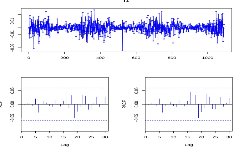
Figure 5: Time series display of the residuals H19I.
3.3 Unit commitment results
3.3.1 Solution using the bounded variable mixed integer linear programming model
6 7 8 9 10 11 12 13 14 15 16 17 18 19 20 21 22 23 24 25 26 27 28 29 30 31 32 33 34 35 36 37 38 39 40 41 42 43 44 45 46 47 48 49 50 51 52 53 54 55 56 57 58 59 60 61
Observation number
Electr
icity demand at 19:00 (MW)
0 50 100 150
22000
24000
26000
28000
30000
32000
34000
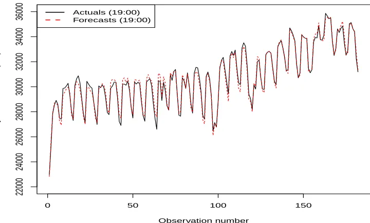
[image:17.612.81.441.155.372.2]36000 Actuals (19:00)Forecasts (19:00)
Figure 6: Plot of actual demand and forecasts.
24000 30000 36000
0.00000
0.00005
0.00010
0.00015
0.00020
0.00025
Electricity demand at 19:00 (MW)
Density
Actuals)
Forecasts(nointeract)
24000 30000 36000
0.00000
0.00005
0.00010
0.00015
0.00020
0.00025
Electricity demand at 19:00 (MW)
Density
Actuals
Forecasts(interact)
[image:17.612.281.445.447.652.2]6 7 8 9 10 11 12 13 14 15 16 17 18 19 20 21 22 23 24 25 26 27 28 29 30 31 32 33 34 35 36 37 38 39 40 41 42 43 44 45 46 47 48 49 50 51 52 53 54 55 56 57 58 59 60 61 62 63 64
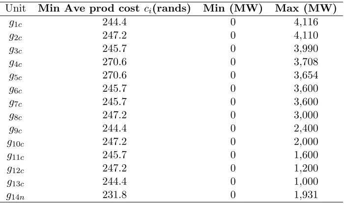
Table 5: Base load demand stations.
Unit Min Ave prod cost ci(rands) Min (MW) Max (MW)
g1c 244.4 0 4,116
g2c 247.2 0 4,110
g3c 245.7 0 3,990
g4c 270.6 0 3,708
g5c 270.6 0 3,654
g6c 245.7 0 3,600
g7c 245.7 0 3,600
g8c 247.2 0 3,000
g9c 244.4 0 2,400
g10c 247.2 0 2,000
g11c 245.7 0 1,600
g12c 247.2 0 1,200
g13c 244.4 0 1,000
g14n 231.8 0 1,931
Table 6: Peaking stations.
Unit Min Ave prod cost ci(rands) Min (MW) Max (MW)
g15g 596.4 0 1,338
g16g 490.6 0 740
g17g 490.6 0 171
g18g 460.8 0 171
g19p 231.2 0 1,000
g20p 231.2 0 400
g21h 231.2 0 344
g22h 231.2 0 240
[image:18.612.136.484.413.538.2]6 7 8 9 10 11 12 13 14 15 16 17 18 19 20 21 22 23 24 25 26 27 28 29 30 31 32 33 34 35 36 37 38 39 40 41 42 43 44 45 46 47 48 49 50 51 52 53 54 55 56 57 58 59 60 61
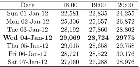
Table 7: Out of sample forecasts (Q0.5 quantile forecasts).
Date 18:00 19:00 20:00
Sun 01-Jan-12 22,581 22,835 24,255
Mon 02-Jan-12 25,306 25,657 26,872
Tue 03-Jan-12 28,192 27,860 28,802
Wed 04-Jan-12 29,069 28,724 29775
Thu 05-Jan-12 29,015 28,658 29,758
Fri 06-Jan-12 28,721 28,522 30,176
Sat 07-Jan-12 27,060 27,288 28,976
The bounded variable mixed integer linear programming model is.
Min Z =
13 X
i=1
cigic+c14g14n+ 18 X
i=15
cigig+ 20 X
i=19
cigip+ 22 X
i=21
cigih (26)
where Z denotes the total cost to be minimized.
Subject to
Load balance constraints 13
X
i=1
gic+g14n+ 18 X
i=15
gig+ 20 X
i=19
gip+ 22 X
i=21
gih=PDht, h= 18,19,20; t= 04/01/2012 (27)
with PD18t= 29,069MW, PD19t= 28,724MW, PD20t= 29,775MW. (28)
The generation reserve margin expressed as a percentage is the method usually used to evaluate the generation system adequacy which is normally in the range 15-25% ([4]). Using a 15% reserve margin we get
PR18t= 0.15×29,069 = 4,360.35MW, PR19t= 0.15×28,724 = 4,308.6MW,
PR20t= 0.15×29,775 = 4,466.25MW (29)
Power reserve constraints
1.15
13 X
i=1
gic+g14n+ 18 X
i=15
gig+ 20 X
i=19
gip+ 22 X
i=21
gih !
≤44,003 (30)
Generator power output limits
0≤g1c≤4,116 (31)
. (32)
6 7 8 9 10 11 12 13 14 15 16 17 18 19 20 21 22 23 24 25 26 27 28 29 30 31 32 33 34 35 36 37 38 39 40 41 42 43 44 45 46 47 48 49 50 51 52 53 54 55 56 57 58 59 60 61 62 63 64
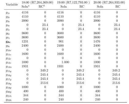
[image:20.612.101.510.218.560.2]The optimal solution for each of the three hours on Wednesday 4 January 2012 is presented in Table 8. Column 2 of Table 8 shows the amount of electricity in megawatts each one of the generating units should produce to meet the predicted demand for that hour at the same time ensuring that the power reserve constraint is met. The minimum cost in rands of producing electricity at each of the three hours is given in parentheses.
Table 8: Optimal Solution using bounded variable MILP
Variable 18:00 (R7,082,499.00) 19:00 (R6,997,215.00 ) 20:00 (R7,257,022.00)
Solna RCb Soln RC Soln RC
g1c 4116 0 4116 0 4116 0
g2c 4110 0 4110 0 4110 0
g3c 3990 0 3990 0 3990 0
g4c 0 23.4 0 23.4 0 23.4
g5c 0 23.4 0 23.4 0 23.4
g6c 3600 0 3600 0 3600 0
g7c 3600 0 3600 0 3600 0
g8c 738 0 393 0 1444 0
g9c 2400 0 2400 0 2400 0
g10c 0 0 0 0 0 0
g11c 1600 0 1600 0 1600 0
g12c 0 0 0 0 0 0
g13c 1000 0 1000 0 1000 0
g14n 1931 0 1931 0 1931 0
g15g 0 349.2 0 349.2 0 349.2
g16g 0 243.4 0 243.4 0 243.4
g17g 0 243.4 0 243.4 0 243.4
g18g 0 213.6 0 213.6 0 213.6
g19p 1000 0 1000 0 1000 0
g20p 400 0 400 0 400 0
g21h 344 0 344 0 344 0
g22h 240 0 240 0 240 0
a
Soln-Solution
b
RC-Reduced cost
The Q0.99 (99th percentile) quantile forecasts are given in Table 9. This means that it is highly
unlikely that electricity demand will exceed 29,562MW, 29,232MW and 29,807MW on hours 18:00, 19:00 and 20:00 respectively on Wednesday 4 January 2012. The expected maximum costs associated
with the Q0.99 quantile forecasts are given in Table 10. This analysis may be useful to power utility
companies such as Eskom with the unit commitment scheduling and economic dispatching of electricity. It is noted that the optimal solutions from Tables 8 and 10 are the same except for generating unit
g8c. This shows that for any increase in demand from the median forecasts (Q0.5 quantile forecasts)
6 7 8 9 10 11 12 13 14 15 16 17 18 19 20 21 22 23 24 25 26 27 28 29 30 31 32 33 34 35 36 37 38 39 40 41 42 43 44 45 46 47 48 49 50 51 52 53 54 55 56 57 58 59 60 61
Table 9: Out of sample forecasts (Q0.99 quantile forecasts)
Date 18:00 19:00 20:00
Sun 01-Jan-12 23,127 23,879 24,718
Mon 02-Jan-12 25,722 26,417 27,085
Tue 03-Jan-12 29,047 28,331 28,862
Wed 04-Jan-12 29,562 29,232 29,807
Thu 05-Jan-12 29,399 29,300 29,912
Fri 06-Jan-12 28,908 29,362 30,300
Sat 07-Jan-12 27,488 28,187 29,019
Table 10: Optimal Solution using bounded variable MILP (forQ0.99 quantile forecasts)
Variable 18:00 (R7,204,369.00) 19:00 (R7,122,793.00 ) 20:00 (R7,264,933.00)
Solna RCb Soln RC Soln RC
g1c 4116 0 4116 0 4116 0
g2c 4110 0 4110 0 4110 0
g3c 3990 0 3990 0 3990 0
g4c 0 23.4 0 23.4 0 23.4
g5c 0 23.4 0 23.4 0 23.4
g6c 3600 0 3600 0 3600 0
g7c 3600 0 3600 0 3600 0
g8c 1231 0 901 0 1476 0
g9c 2400 0 2400 0 2400 0
g10c 0 0 0 0 0 0
g11c 1600 0 1600 0 1600 0
g12c 0 0 0 0 0 0
g13c 1000 0 1.000 0 1000 0
g14n 1931 0 1931 0 1931 0
g15g 0 349.2 0 349.2 0 349.2
g16g 0 243.4 0 243.4 0 243.4
g17g 0 243.4 0 243.4 0 243.4
g18g 0 213.6 0 213.6 0 213.6
g19p 1000 0 1000 0 1000 0
g20p 400 0 400 0 400 0
g21h 344 0 344 0 344 0
g22h 240 0 240 0 240 0
[image:21.612.97.517.321.661.2]6 7 8 9 10 11 12 13 14 15 16 17 18 19 20 21 22 23 24 25 26 27 28 29 30 31 32 33 34 35 36 37 38 39 40 41 42 43 44 45 46 47 48 49 50 51 52 53 54 55 56 57 58 59 60 61 62 63 64
4
Conclusion
The paper presented an application of partially linear additive quantile regression models to short term electricity demand forecasting using South African data. The study focused on the peak hours of the day. Variable selection was done using Lasso via hierarchical pairwise interactions. Models for each hour were split into one with and one without pairwise interactions. Models of each hour were combined using an algorithm in which the average loss suffered was based on the pinball loss function. This resulted in three sets of forecasts for each hour. The best set of forecasts was selected based on probabilistic forecast error measures, pinball loss values, continuous ranked probability scores and the log scores. For instance, as shown in 2 the model without interactions has smaller pinball loss value as compared to the other two models considered for hour 18:00 and was found to be the best fitting model. while from hours 19:00 and 20:00 model with interactions and the combined model were the best fitting models respectively.
The forecasts from the three hours were then used as inputs in solving the unit commitment prob-lem. A bounded variable mixed integer programming modelling approach was used and the developed optimization models were solved using Lingo version 14. Median forecasts for Wednesday 4 January 2012 were 29,069MW, 28,724MW and 29,775MW for the hours 18:00, 19:00 and 20:00respectively, with the corresponding optimal minimal costs of R7,082,499.00, R6,997,215.00 and R7,257,022.00. Results from the unit commitment problem show that it is very costly to use gas fired generating
units. These were not selected as part of the optimal solution. Using theQ0.99 quantile forecasts, it
is noted that the optimal solutions from median forecasts (Q0.5 quantile forecasts) are the same as
those from theQ0.99 quantile forecasts except for generating unit g8c, which is a coal fired unit. This
shows that for any increase in demand from the median forecasts it will be economical to increase
the generation of electricity from generating unit g8c. The Q0.99 quantile forecasts for
Wednes-day 4 January 2012 for the hours 18:00, 19:00 and 20:00 were found to be 29,562MW, 29,232MW and 29,807MW respectively with optimal solutions of R7,204,369.00, R7,122,793.00 and R7,264,933.00
The main contribution of this study is in the use of nonlinear trend variables and the combining of forecasting with the unit commitment problem. The study could be useful to system operators in power utility companies in scheduling and dispatching of electricity at a minimal cost particularly during the peak period when the grid is constrained due to increased demand for electricity. Future work could look at peak load forecasting where the extreme peaks could be used in the assessment of power system reliability [4] including the use of stochastic programming techniques which are known to capture a lot of uncertainties in the unit commitment problem. The modelling framework discussed in this paper can also be used in solar power forecasting with similar input variables.
Acknowledgments
6 7 8 9 10 11 12 13 14 15 16 17 18 19 20 21 22 23 24 25 26 27 28 29 30 31 32 33 34 35 36 37 38 39 40 41 42 43 44 45 46 47 48 49 50 51 52 53 54 55 56 57 58 59 60 61
Appendix
Appendix A1: Evaluating the prediction errors
[image:23.612.212.409.250.306.2]Tables 11 - 13 show the accuracy measures, root mean square error (RMSE), mean absolute error (MAE) and mean absolute percentage error (MAPE) for each of the models used for electricity demand at hours 18:00, 19:00 and 20:00 respectively. These error measures are generally used for predicting point forecasts.
Table 11: Model comparisons with and without interactions: Hour 18:00 (Q0.5)
M1 M2 M3
RMSE 353.05 354.54 352.63
MAE (MW) 293.10 294.62 293.30
MAPE (%) 0.9706 0.9710 0.9697
Table 12: Model comparisons with and without interactions: Hour 19:00 (Q0.5)
M4 M5
RMSE 306.69 290.49
MAE (MW) 244.36 232.78
MAPE (%) 0.8093 0.7736
Table 13: Model comparisons with and without interactions: Hour 20:00 (Q0.5)
M6 M7 M8
RMSE 350.78 327.85 326.89
MAE (MW) 280.64 251.20 253.40
MAPE (%) 0.9189 0.8242 0.8308
Appendix A2: Plots of forecasted demand for hours 18:00 and 20:00
6 7 8 9 10 11 12 13 14 15 16 17 18 19 20 21 22 23 24 25 26 27 28 29 30 31 32 33 34 35 36 37 38 39 40 41 42 43 44 45 46 47 48 49 50 51 52 53 54 55 56 57 58 59 60 61 62 63 64
Observation number
Daily peak electr
icity demand (MW)
0 50 100 150
22000
24000
26000
28000
30000
32000
34000
[image:24.612.82.443.154.372.2]36000 ActualsForecasts (combined)
Figure 8: Plot of actual demand and combined forecasts (18:00)
25000 30000 35000
0.00000
0.00005
0.00010
0.00015
0.00020
0.00025
Electricity demand at 18:00 (MW)
Density
Actuals
Forecasts(combined)
25000 30000 35000
0.00000
0.00005
0.00010
0.00015
0.00020
0.00025
Electricity demand at 18:00 (MW)
Density
Actuals
[image:24.612.272.440.447.653.2]Forecasts(nointer)
6 7 8 9 10 11 12 13 14 15 16 17 18 19 20 21 22 23 24 25 26 27 28 29 30 31 32 33 34 35 36 37 38 39 40 41 42 43 44 45 46 47 48 49 50 51 52 53 54 55 56 57 58 59 60 61
Observation number
Electr
icity demand at 20:00 (MW)
0 50 100 150
22000
24000
26000
28000
30000
32000
34000
[image:25.612.80.442.156.371.2]36000 Actuals (20:00)Forecasts (20:00)
Figure 10: Plot of actual demand and forecasts (20:00)
24000 30000 36000
0.00000
0.00010
0.00020
0.00030
Electricity demand at 20:00 (MW)
Density
Actuals)
Forecasts(nointeract)
24000 30000 36000
0.00000
0.00010
0.00020
0.00030
Electricity demand at 20:00 (MW)
Density
Actuals
Forecasts(interact)
[image:25.612.283.444.448.652.2]6 7 8 9 10 11 12 13 14 15 16 17 18 19 20 21 22 23 24 25 26 27 28 29 30 31 32 33 34 35 36 37 38 39 40 41 42 43 44 45 46 47 48 49 50 51 52 53 54 55 56 57 58 59 60 61 62 63 64
References
[1] Almeshaiei E., Soltan H. A methodology for electric power load forecasting. Alexandria Engineer-ing Journal 2011; 50:137–144.
[2] Amina M, Kodogiannis VS, Petrounias I, Tomtsis D. A hybrid intelligent approach for the pre-diction of electricity consumption. Electrical Power and Energy Systems 2012; 43:99–108.
[3] Bien J, Taylor J, Tibshirani R. A lasso for hierarchical interactions. The Annals of Statistics 2013; 41(3): 1111–1141.
[4] ˇCepin M. Assessment of power system reliability: Methods and applications. London: Springer,
2011.
[5] Chikobvu D, Sigauke C. Modelling influence of temperature on daily peak electricity demand in South Africa. Journal of Energy in Southern Africa 2013; 24(4):63–70.
[6] Dai H, Zhang N, Su W. A literature review of stochastic programming and unit commitment. Journal of Power and Energy Engineering 2015; 3:206–214.
[7] Devaine M, Gaillard P, Goude Y, Stoltz G. Forecasting the electricity consumption by aggregating specialized experts; a review of sequential aggregation of specialized experts, with an application to Slovakian and French country-wide one-day-ahead (half-) hourly predictions, Machine Learning 2012; 90: 231-260.
[8] Engle R F, Granger C W J, Rice J, Weiss A. Semiparametric estimates of the relation between weather and electricity sales. Journal of the American Statistical Association 1986; 81: 310–320.
[9] Fahad MU, Arbab N. Factor affecting short term load forecasting. Journal of Clean Energy Technologies 2014; 2(4):305–309.
[10] Fan S, Hyndman RJ. Short term load forecasting based on a semiparametric additive model. IEEE Transactions on Power Systems 2012; 27(1):134–141.
[11] Fasiolo M, Goude Y, Nedellec R, Wood S N. Fast calibrated additive quantile regression 2017.
Available at https://arxiv.org/abs/1707.03307
[12] Feng Y, Ryan SM. Day-ahead hourly electricity load modeling by functional regression. Applied Energy 2016; 170: 455–465.
[13] Gaillard P, Goude Y, Nedellec R. Semi-parametric models and robust aggregation for GEF-Com2014 probabilistic electric load and electricity price forecasting. International Journal of Forecasting 2016; 32(3): 1038–1050.
[14] Gibbons CE, Faruqui A. Quantile Regression for Peak Demand Forecasting. Available at SSRN
2014; https://papers.ssrn.com/sol3/papers.cfm?abstract_id=2485657. (accessed on 8
De-cember 2016).
[15] Gneiting T, Katzfuss M. Probabilistic forecasting, Annual Review of Statistics and Its Application 2014; 1, 125–151.
6 7 8 9 10 11 12 13 14 15 16 17 18 19 20 21 22 23 24 25 26 27 28 29 30 31 32 33 34 35 36 37 38 39 40 41 42 43 44 45 46 47 48 49 50 51 52 53 54 55 56 57 58 59 60 61
[17] Hastie TJ, Tibshirani RJ. Generalized Additive Models. London:Chapman and Hall, 1990.
[18] He Y, Liu R, Li H, Wang S, Lu X. Short-term power load probability density forecasting method using kernel-based support vector quantile regression and copula theory. Applied energy 2017; 185: 254–266.
[19] Hinman J, Hickey E. Modelling and forecasting short-term electricity load using regression anal-ysis. Institute of Regulatory Policy Studies 2009; 1–51.
[20] Hong T, Fan S. Probabilistic electric load forecasting: A tutorial review. International Journal of Forecasting 2016; 32(3): 914–938.
[21] Hong T, Pinson P, Fan S, Zareipour H, Troccoli A, Hyndman RJ. Probabilistic energy forecasting: Global Energy Forecasting Competition 2014 and beyond. International Journal of Forecasting 2016; 32(3): 896–913.
[22] Hong T, Wang P, White L. Weather station selection for electric load forecasting. International Journal of Forecasting 2015; 31:286 295.
[23] Hoshino T. Quantile regression estimation of partially linear additive models. Journal of Non-parametric Statistics 2014; 26(3): 509–536.
[24] Hu Y, Zho K, Lian H. Bayesian quantile regression for partially linear additive models. Statistics and Computing 2015; 25(3):651–668.
[25] Hyndman RJ. and Athanasopoulos G. Forecasting: principles and practice. OTexts, 2013.
[On-line]. Available: https://www.otexts.org/fpp
[26] Janicki M. Methods of weather variables introduction into short-term electric load forecasting
models - a review. 2017 [Online]. Available: http://DOI:10.15199/48.2017.04.18
[27] James G, Witten D, Hastie T, Tibshirani R. An Introduction to Statistical Learning: with Ap-plications in R. Springer 2015.
[28] Jiang YL. Double-Penalized Quantile Regression in Partially Linear Models. Open Journal of Statistics 2015; 5: 158-164.
[29] Koenker R, Bassett GW. Regression quantiles. Econometrica 1978; 46:33–50.
[30] Koenker R. Quantile Regression. Cambridge University Press, 2005.
[31] Kurban M., Filik U.B. Unit commitment scheduling by using the autoregressive and artificial neural network models based short-term load forecasting. In: Probabilistic methods applied to power systems 2008; IEEE: 1–5.
[32] Lim M, Hastie T. Learning interactions via hierarchical group-lasso regularization. J Comput Graph Stat. 2015, 24(3): 627–654.
[33] Odhiambo NM. Energy consumption, prices and economic growth in three SSA countries: A comparative study. Energy Policy 2010; 38:2463–2469.
6 7 8 9 10 11 12 13 14 15 16 17 18 19 20 21 22 23 24 25 26 27 28 29 30 31 32 33 34 35 36 37 38 39 40 41 42 43 44 45 46 47 48 49 50 51 52 53 54 55 56 57 58 59 60 61 62 63 64
[35] Olusegun AM, Dikko HG, and Gulumbe SU. Identifying the limitation of stepwise selection for variable selection in regression analysis. American Journal of Theoretical and Applied Statistics 2015, 4(5):414 419.
[36] Portnoy S, Koenker R. The Gaussian Hare and the Laplacian Tortoise: Computability of Squared-Error versus Absolute-Squared-Error Estimators. Statistical Science 1997; 12(4): 279–296.
[37] Power Generation Technology Data for Integrated Resource Plan of South Africa. EPRI,
Palo Alto, CA: 2015. (Accessed on 21 October 2017). http://www.energy.gov.za/IRP/2016/
IRP-AnnexureA-EPRI-Report-Power-Generation-Technology-Data-for-IRP-of-SA.pdf
[38] Saravanan B, Das S, Sikri S, Kothari DP. A solution to the unit commitment problem-a review. Front Energy 2013; 7(2):223–236.
[39] Sigauke C. Modelling electricity demand in South Africa, PhD Thesis, University of the Free-State 2014.
[40] Short M, Crosbie T, Dawood M, Dawood N. Load forecasting and dispatch optimisation for decentralised co-generation plant with dual energy storage. Applied Energy 2017; 186: 304–320.
[41] Taieb SB, Huser R, Hyndman RJ., Genton MG. Forecasting uncertainty in electricity smart meter data by boosting additive quantile regression. IEEE Transactions on Smart Grid 2016; 7(5): 2448–2455.
[42] Taylor JW, McSharry PE. Short term load forecasting methods: An evaluation based on european data. IEEE Transactions on Power Systems 2008; 22:2213–2219.
[43] Tibshirani R. Regression shrinkage and selection via the Lasso. Journal of the Royal Statistical Society B 1996; 58(1): 267–288.
[44] Wood SN. Generalized Additive Models: An introduction with R. London: Chapman and Hall, 2006.
[45] Wright B. A review of unit commitment 2013; http://blog.narotama.ac.id/wp-content/
uploads/2014/12/A-Review-of-Unit-Commitment.pdf (accessed 26 June 2017).
[46] Wu L, Shahidehpour M, Li T. Stochastic Security-Constrained Unit Commitment. IEEE Trans-actions on Power Systems 2007, 22(2):800–811.
[47] Xia C., Wan J., McMenemy K. Short, medium and long term load forecasting model and virtual load forecaster based on radial basis function neural networks. Electrical Power and Energy Systems 2010; 32:743–750.
Daily peak electr
icity demand (MW)
22000
24000
26000
28000
30000
32000
34000
25000
30000
35000
0.00000
0.00005
0.00010
0.00015
0.00020
0.00025
Density
Actuals
Forecasts(combined)
25000
30000
35000
0.00000
0.00005
0.00010
0.00015
0.00020
0.00025
Density
Actuals
Electr
icity demand at 20:00 (MW)
22000
24000
26000
28000
30000
32000
34000
24000
30000
36000
0.00000
0.00010
0.00020
0.00030
Density
Actuals)
Forecasts(nointeract)
24000
30000
36000
0.00000
0.00010
0.00020
0.00030
Density
Actuals
●
● ●
● ● ●
● ●
● ● ●
● ● ●
● ●
● ● ● ● ● ●
● ● ●
●
● ● ● ●
● ●
●