DEPARTMENT OF COMPUTER AND
MA THEMA
TI CAL SCIENCES
The Optimal Sampling Point for the Quality Assessment
of Continuous Streams
Neil S. Barnett IanS. Gomm
Len Armour
(31EQRM11) August 1993
·
TECHNICAL
REPORT
VICTORIA UNIVERSITY OF TECHNOLOGY (P 0 BOX 14428) MELBOURNE MAIL CENTRE
MELBOURNE, VICTORIA, 3000 AUSTRALIA
THE OPTIMAL SAMPLING POINT FOR THE
QUALITY ASSESSMENT OF CONTINUOUS
STREAMS
NEIL S. BARNETT, IAN S. GOMM, LEN ARMOUR
Victoria University of Technology
Summary
Attention is drawn to the need to consider the point of sampling in situations where a single sample is used to estimate the mean flow of a continuous stream. When the flow rate is varying and where the stochastic process, representing the quality characteristic of the
stream, has a linear or exponential variogram, the extent of variation in the location of the optimal sampling point is illustrated using linear and exponential flow rate models and some numerical examples.
Key words: Varying flow rate; linear and exponential variograms; estimation error variance; optimal sampling point; continuous time stochastic process.
1. Introduction
Many industrial applications of statistics are related to issues of
process evaluation, process improvement, process control and
quality assessment. In fact, the current hightened interest in quality
management has fostered a growth in the use of statistical
Companies manufacturing continuous or flowing streams of product typically, if their processes are not totally automated, sample at regular time intervals for the purposes of monitoring and control. Sampling at regular times is frequently preferable to other sampling strategies because it is organisationally convenient both from the perspective of collecting samples and for scheduling laboratory tests. This regime is sometimes interupted, however, when sample test values of one or more particular product characteristics indicate that further appraisal or corrective action is necessary. Sets of generated sample test results, which are likely to be highly correlated, are frequently used collectively to describe the quality of the product over a particular manufacturing period. From the perspective of
maintaining control of the process, it is usually individual test values that are of prime concern. With this in mind, it is important to
consider how well individual sample test values apprais~ the performance of the process over the time interval which they represent. It is often sufficient that a single test value is a good representative of the mean of an important product characteristic over a period equal in length to the sampling interval.
Specifically, given a fixed sampling interval, and the fact that the mean of a characteristic of the continuous stream, over a period equal in length to the sampling interval is to be estimated by a single sample test value, then where in the interval is the best point to
sample? This paper represents a response to this question, taking the optimal point to mean the point at which the estimation error
2. Assumptions and Practical Context
Use of the term, 'sampling point' reflects the assumption that a
product sample can be collected instantaneously, or at least in a time
interval that is negligable compared with the time between
commencing the collection of successive samples. The location of the
optimal sampling point depends on the flow pattern in the particular
interval and on the stochastic behaviour of the product characteristic
over the same period. It is assumed, in the following, that the flow
pattern is deliberate and deterministic. It is also assumed to be monotonic within the given interval. The situation under
consideration is typified by processes whose throughputs are
progressively increased to a maximum as manufacturing parameters
approach their optimal performance level. Three flow rate patterns
will be considered, constant flow, linear flow and negative
exponential flow. A likely practical production cycle can be
approximately represented by a linearly increasing flow rate from
zero to a constant level, maintenance at this level for a period and
then by a linearly decreasing flow rate to zero.Two adjacent stages
can be treated as a single one by using an exponential approximation.
The actual product characteristic of concern , X(t) which can be
considered to define the quality of the product at time t, is a
continuous time stochastic process which may indeed be
non-stationary. Optimality of location of the sampling point will be
obtained on the basis of achieving minimum error variance for
using just a single sample value taken within the interval. It has been
shown, for example by Saunders et al (1989), that for essentially
constant flows, the error variance is totally expressible in terms of the
variogram of X(t). When the flow rate is deterministic and
independent of X(t), this characteristic is preserved. In the
subsequent analysis, therefore, it is only necessary to make
stipulations about the form of the variogram of the process, X(t). It
should be noted, as pointed out by Robinson (1990), that the
variogram can be stationary even when the stochastic process itself is
non-stationary. Two cases of stochastic process will be considered in
conjunction with the flow patterns described above, one having a
stationary linear variogram and the other having a stationary
exponential variogram.
The assumed deterministic nature of the flow pattern is, of
course, n6t a realistic representation of every situation that can occur
in practice. Other possible scenarios include those where the actual
throughput flow rate itself is a stochastic process and under these
circumstances it may well be necessary to consider the flow and
quality characteristic as a joint stochastic process in continuous ti.me.
Another variant is the continuously monitored process, for which the
flow rate is subject to automatic adjustment in order to accommodate
other changes taking place in operations.
3. Fundamentals
as:-1
V(u)
=
-E[(X(t)-X(t+ u))2]. 2Clearly, V(O)
=
O and V(-u)=
V(u). It would be expected also, that V(u) isstrictly increasing. When X(t) is stationary then
V(u) = cr2 - Cov(u),
where cr2 is the process variance and
Cov(u) the process covariance of
lag u . If the mean characteristic of the flow over the interval ( which
is equal in length to the sampling interval) is denoted by
x
andassuming, without loss of generality, that the period over which it is
desired to estimate this mean is (O,d), then the error variance
resulting from estimating the mean by a single observation, X(t)
taken at time t (O < t < d) is given by, E[(X -X(t))2]. The remainder of
this paper, having developed an expression for this, deals with
finding the values of t that minimize it for five combinations of flow
rate function and process variogram.
4.1 Case (i): Constant Flow Rate, Stationary Variogram
Clearly,
1 d 1 d d
E[(X -X(t))2] = E[(-
J
X(u)du-X(t))2] = -2 E[jf
(X(u)-X(t))(X(v)-X(t))dudv]d 0 d 0 0
and using an identity provided by Saunders et al (1989), this reduces
to:-1 d d 2 d
- -2 J J V(v-u)dudv+-J V(u-t)du
d 0 0 d 0
1 d d 2 t d-t
= - -2 J J V(v-u)dudv+-{J V(u)du+ J V(u)du}.
d 00 d 0 0
Equating to zero the derivative of this, with respect to t, gives,
V(t) = V(d-t)
and hence the optimal sampling location at t =
o.
5d, irrespective of the form of the process variogram.4.2 Non-constant flows:
For situations where the flow rate at time t is some function of t , Y(t)
units of volume (or mass) per unit of time, then
d
J Y(u)X(u)du d
E[(X-X(t))2]=E[(0
d -X(t))2]= d l E[(JY(u)(X(u)-X(t))du)2] ,
J Y(u)du Cf Y(u)du)2 0
0 0
d
where J Y(u)du is the total volume (or mass) of the product
0
throughput in the interval (O,d),
d d
- d l E[f J Y(u)Y(v)(X(u)- X(t))(X(v)-X(t))dudv],
Cf
Y(u)du)2 0 00
1 d d
- d J J Y(u)Y(v)(-V(u-v)+ V(u-t)+ V(v-t))dudv.
Cf
Y(u)du)2 0 0The optimal sampling point is thus given by solving the
equation:-d t d-t
-{JY(t-u)V(u)du+ Jrcu+t)V(u)du}=O ... (1)
dt 0 0
4.3 Case (ii): Linear Flow Rate, Linear Variogram.
Let the flow rate function be Y(t) =Ct+ D,
o
<ts d where there are twodistinct cases, (a) Os C,D and Cd+ D s K, where K is the maximum
possible flow rate and (b)
c
< O,D > O and -Cds
Ds
K. Cases (a) and (b)correspond respectively to increasing (and constant) and decreasing
rates of flow over (0, d).
If the variogram is denoted by V(t) =A+ Bt for t > O and with A,B > O
then (1) becomes,
d t t d-t d-t
-{(Ct+ D)
J
(A+ Bu)du-cf (Au+ Bu2)du+(Ct+D) J
(A+ Bu)du+CJ
(Au+ Bu2)du} =0
dt 0 0 0 0
giving, the equation Ct2+2Dt-d(D+ Cd)=O which has solutions, 2
t=
-D±~D'+Cd(D+ ~d)
when
c
:;t 0c
and t= d when C=O.
2
For case (ii)(a), it can be seen that there is only one positive solution
in (0, d) lying between t =
~
and t = d. For case (ii)(b) there is just onebetween t =
o
and t = d . It should be noted that neither parameters of2
the variogram appear in the expression that gives the optimal
sampling point. When D=
o,
the solution can be seen tobet=~
·
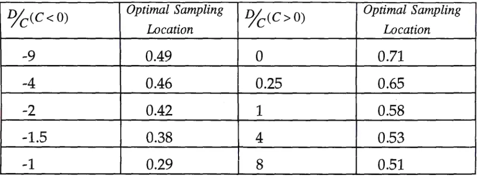
Table 1. Some Numerical
Results:-Let K = 1
o
tonnes per hour and d = 1 hour,o/cCC< 0) Optimal Sampling o/cCC> 0) Optimal Sampling
Location Location
-9 0.49 0 0.71
-4 0.46 0.25 0.65
-2 0.42 1 0.58
-1.5 0.38 4 0.53
I
-1 0.29 8 0.51
4.4 Case (iii): Linear Flows, Exponential variogram.
Let the flow rate function be as defined for case (ii) and the
variogram be of the form,
V(u) =A+ B(l-e-Eu) for E > 0 and A,B > 0.
Again, applying equation (1) and simplifying, the following
quadratic equation is obtained,
providing the solutions Y =
C±~C
2 +(ED-C)(DE+dCE+C)e-Ed e-Ed (DE+ dCE + C)For the case where
c
=o
the solution t = d is retrieved.2
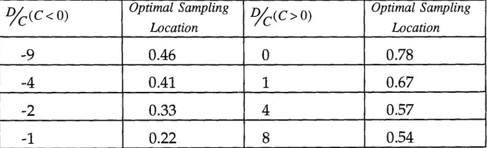
Table 2. Some Numerical
Results:-Let K = 10 tonnes per hour, d = 1 hour and E = 5,
o/cCC < O) Optimal Sampling o/cCC>O) Optimal Sampling
Location Location
-9 0.46 0 0.78
-4 0.41 1 0.67
-2 0.33 4 0.57
-1 0.22 8 0.54
4.5 Case (iv): Exponential Flow Rate, Linear Variogram.
Let the flow rate function be given
by:-Y(t)=C+(K-C)(l-e-v1
) with 05'C5'K and D'2:.0,
which is the case of increasing (and constant) flow rate over the
interval (O,d). Let the variogram be defined as in case (ii). Applying
-Dt DK 1 (1 dDK -Dd e + t - - + +e ) = 0
(K - C) 2 (K - C) I
which can be solved numerically, for example by using the method
of Newton-Raphson. For the case where
c
=o
this reduces to,e-Dt + Dt-_!_(I +dD+e-Dd) =
o
which can be shown, for the constraints 2assumed on the parameters, to have a single solution in the interval
(0, d) and lying to the right of centre.
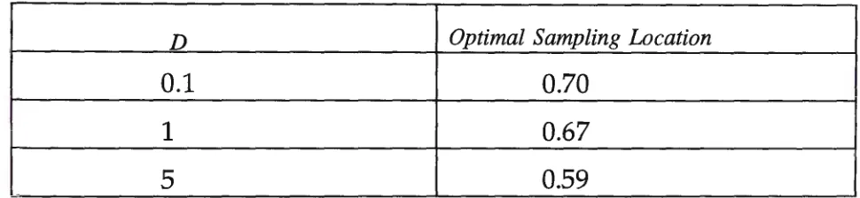
Table 3. Some Numerical
Results:-Let K
=Io
tonnes per hour and d=I
hour andc = o,
D Optimal Sampling Location
0.1 0.70
1 0.67
5 0.59
4.6 Case (v): Exponential Flow Rate, Exponential Variogram.
Let the flow rate be defined as in case (iv) and the variogram as in
case (iii) with the added condition that D -:F-E. Application of equation
(1) yields,
eEt e-Ed (D-E)(K(D + E)-(K - C)Ee-dD )- e-Et (D + E)(KD- CE)+ 2e-vr (K - C)ED = 0
When
c
=Kor D = O or D--::, oo this reduces to case (i). As in case (iv), aWhen D=E application of equation (1) yields,
e2Dce-Dd (2K -(K -C)e-Dd)-2D(K -C)t-C-K = 0.
Table 4. Some Numerical
Results:-Let K
=
10 tonnes per hour and d=
1 hour,c
=
o
and E=
1D Optimal Sampling Location
0.1 0.72
1 0.69
2 0.66
5 0.60
5. Concluding Remarks
The variation in the location of the optimal sampling point, for mean
flow estimation, has been demonstrated using some flow rate and
variogram models that have some practical merit. For a
monotonically increasing flow rate, the optimal sampling point
moves to the right of the interval centre and for a monotonically
decreasing one, it moves to the left of centre. It follows then, that for
situations where the rate of process throughput is largely regulated,
there may well be a case for carefully considering the time at which
samples are taken, particularly in the 'warm-up' and 'close-down'
periods. From a practical stand-point, a decision on the sampling
greater error variance by virtue of not sampling at the optimal point. For case (i), for example, when the process variogram is linear and the flow rate constant, the estimation error variance varies between
Bd d 2Bd d d" h . th 1 . k
A+
6
an A+-3- epen mg on w ere m (O,d) e samp e 1s ta en.References
ROBINSON, G.K. (1990). A Role for Variograms. Austral. J. Statist., 32, 327-335.
SAUNDERS, I.W., ROBINSON, G.K., LWIN, T., HOLMES, R.J. (1989). A Simplified
Variogram Method for the Estimation Error Variance in Sampling from a Continuous