warwick.ac.uk/lib-publications
Original citation:
Leng, Chenlei and Pan, Guangming (2018) Covariance estimation via sparse Kronecker
structures. Bernoulli, 24 (4B). pp. 3833-3863. doi:
10.3150/17-BEJ980
Permanent WRAP URL:
http://wrap.warwick.ac.uk/91297
Copyright and reuse:
The Warwick Research Archive Portal (WRAP) makes this work by researchers of the
University of Warwick available open access under the following conditions. Copyright ©
and all moral rights to the version of the paper presented here belong to the individual
author(s) and/or other copyright owners. To the extent reasonable and practicable the
material made available in WRAP has been checked for eligibility before being made
available.
Copies of full items can be used for personal research or study, educational, or not-for-profit
purposes without prior permission or charge. Provided that the authors, title and full
bibliographic details are credited, a hyperlink and/or URL is given for the original metadata
page and the content is not changed in any way.
A note on versions:
The version presented in WRAP is the published version or, version of record, and may be
cited as it appears here.
https://doi.org/10.3150/17-BEJ980
Covariance estimation via sparse Kronecker
structures
C H E N L E I L E N G1and G UA N G M I N G PA N2
1Department of Statistics, University of Warwick, Coventry CV4 7AL, UK. E-mail:[email protected] 2School of Physical and Mathematical Sciences, Nanyang Technological University, Singapore 637371,
Republic of Singapore. E-mail:[email protected]
The problem of estimating covariance matrices is central to statistical analysis and is extensively addressed when data are vectors. This paper studies a novel Kronecker-structured approach for estimating such ma-trices when data are mama-trices and arrays. Focusing on matrix-variate data, we present simple approaches to estimate the row and the column correlation matrices, formulated separately via convex optimization. We also discuss simple thresholding estimators motivated by the recent development in the literature. Non-asymptotic results show that the proposed method greatly outperforms methods that ignore the matrix struc-ture of the data. In particular, our framework allows the dimensionality of data to be arbitrary order even for fixed sample size, and works for flexible distributions beyond normality. Simulations and data analysis further confirm the competitiveness of the method. An extension to general array-data is also outlined.
Keywords:covariance matrix; Kronecker structure; matrix data; non-asymptotic bound
1. Introduction
Matrix and array observations are becoming increasingly available in the big data era thanks to the rapid advance in the information technology and the need to store data in structured forms; see, for example, Li, Kim and Altman [14], Hoff [11], Leng and Tang [13], Zhou, Li and Zhu [24], and Zhou et al.[25]. Consider independent and identically distributed matrix-variates X1, . . . , Xn ∈Rp×q that are realizations of a matrix random variable X following a
matrix-variate distribution (Gupta and Nagar [10]). Writing vec as the vector operator that stacks the columns of a matrix into a vector, we denote
varvec(Xk)
=
as thepq×pqdimensional covariance matrix. Without loss of generality, we assume that E(Xk)
is known or a consistent estimator of E(Xk)such as the sample mean is available. For the latter
case, we requiren >1. In the sequel, we work withXk−E(Xk).
The covariance matrix plays an indispensable role in multivariate data analysis and is a central quantity for estimation and inference. To begin with, a simple estimate of is the fa-miliar sample covariance matrix after these observations are vectorized. However, whenever the data dimensionpqis larger than the sample sizen, this estimator can be of little use due to its singularity. Based on this observation, a plethora of approaches, built upon various sparsity as-sumptions on, have attracted increasing attention. See, for example, Bickel and Levina [3,4],
Rothman, Levina and Zhu [17], Cai and Liu [6], Bien and Tibshirani [5], Rothman [15], Xue, Ma and Zou [21], and Cui, Leng and Sun [8].
Stacking matrices into vectors incurs a loss of information in the matrix form of the data. An attractive alternative is to assume (Hoff [11], Leng and Tang [13], Tsiligkaridis and Hero [19])
=⊗,
where, loosely speaking, =(ψij)∈Rq×q depicts the covariance of the columns ofXi and
=(σij)∈Rp×pthat of the rows. Using a Kronecker product for the overall covariance matrix
retains the matrix structure of the data. Another immediate advantage is that the number of the unknown parameters inreduces from an order ofp2q2to an order ofp2+q2, making the prob-lem more tractable. As will become clear, with appropriate sparsity assumptions onand, this decomposition enables one to estimateat a higher rate of convergence, and allows substantially larger dimensional covariances to be estimated, even with a fixed sample size. Without consider-ing sparsity, Srivastava, von Rosen and von Rosen [18] estimated the Kronecker structure when p andq are fixed. There are also a growing number of papers on estimating the concentration matrix−1via a Kronecker product representation by estimating sparse concentration matrices −1and−1(Allen and Tibshirani [1], Yin and Li [22], Leng and Tang [13], Zhou [26]). These papers assume matrix normality for the data distribution. None of them addresses the issue of estimating sparse or.
usually suffice to guarantee its positive definiteness in contrast to the thresholding estimator for the covariance matrix of vector data where special care is recommended (Rothman [15], Xue, Ma and Zou [21]). This is in sharp contrast to the more difficult problem of estimation concentration matrices where loss function based approaches have to be employed (Leng and Tang [13]).
The following notations are used throughout the paper. For a square matrixA=(aij)∈Rm×m,
diag(A) denotes a matrix consisting of the diagonal terms of A as diag{a11, . . . , amm}. The
Frobenius norm ofAis denoted asAF and its element1norm is denoted as|A|1. We write
|A|max=maxi,j|aij|as the maximum entry ofA. The spectral norm ofAisA2denoting the
largest singular value ofA. The trace of a square matrixAis denoted as tr(A)and the Kronecker product between matrices is denoted by⊗. A positive semi-definite matrix is denoted byA0. The(i, j )th entry of A is denoted either asaij or Aij. IfA denotes a covariance matrix, the
corresponding correlation matrix is denoted asRA such that{diag(A)}1/2RA{diag(A)1/2} =A. Finally,Ikdenotes thek×kidentity matrix.
The rest of the paper is organised as follows. We present the proposed Kronecker-structured es-timation method in Section2, where several variants of the approach are discussed. In Section3, we provide the main theory, and outline the generalisation of the proposed method for estimat-ing the covariance matrix of array data. Simulation studies and data analysis are presented in Section4with a short conclusion in Section5. All the proofs are relegated to theAppendix.
2. Kronecker-structured estimation
We make the following assumption on the matrix variate dataXthat includes multivariate nor-mality as a special case.
Condition (A). The matrix variate dataXhave the structure
X=BSAT, (1)
whereA,Bare square matrices such thatAAT=,BBT=and the entries ofS=(sij)are
independent and identically distributed with mean 0 and variance 1.
First we derive a simple sample estimate for=⊗. Write
n=
1 n
n
k=1
XTkXk, n=
1 n
n
k=1
XkXkT.
Clearly, the expectations of these two matrices satisfy
E(n)=tr(), E(n)=tr(),
respectively, giving rise to a reasonable estimate of=⊗asn⊗n/(tr()tr()). Noting
a simple sample estimate ofadmitting the Kronecker structure is
n=n⊗n/
1 n
n
k=1
Xk2F
. (2)
If the sample size goes to infinity and the dimensionality of the covariance matrix is fixed, it is not difficult to see thatnis a consistent estimator of.
Next, we discuss how to estimatewhenpandqare much larger thann. Define the marginal variance matrices ofnandnas
W12=diag(n),
W12=diag(n),
respectively. The sample row and column sample correlation matrices can be written respectively asRn andRn, where
n=W1RnW1, n=W1RnW1.
These two sample correlation matrices can be seen as estimates of the population correlation matricesR andR, respectively. The proposed Kronecker estimator replacesRnandRnby their penalized estimates in
R=arg min
R∈Rq×q 1 2 R−R
n
2
F +λ|R|1, s.t.R Iq, Rjj=1, j=1, . . . , q, (3)
R=arg min
R∈Rp×p 1 2 R−R
n
2
F +λ|R|1, s.t.R Ip, Rjj=1, j=1, . . . , p, (4)
whereλandλare penalty parameters, and is an arbitrary small positive constant that
guar-antees positive definiteness of the estimates. Here the simplified notationR(R) suppresses its dependence on the sample sizenand the penalty parameterλ(λ). The optimization problem
in (3) and (4) is convex and thus convex optimization techniques can be applied. In this paper, we use the efficient accelerated proximal gradient algorithm in Cui, Leng and Sun [8]. After obtaining the penalized estimates ofand, the final Kronecker estimator assembles them as
=W1RW1, =W1RW1, =⊗/
1 n
n
k=1
Xk2F
. (5)
Motivated by the adaptive Lasso (Zou [27]), we can replace the penalty |R|1 in (3) by
j <k|Rj k|/|(Rn)j k|, and the penalty in (4) by
j <k|Rj k|/|(Rn)j k|. After the correlation
ma-trices are obtained, we estimate,andas in (5). The estimate is denoted asˆAand referred to as the adaptive Kronecker estimator.
estimating theq×qmatrix, the effective sample size becomesnp. Thus, the curse of dimen-sionality is greatly alleviated. As a consequence, we can directly use thresholding as in in Bickel and Levina [4] and Rothman, Levina and Zhu [17] without the positive definite constraints, giv-ing rise to simple and fast estimators. Although thresholdgiv-ing estimators for covariance of vector data are also found to be positive definite with high probability (Bickel and Levina [4], Rothman, Levina and Zhu [17]), in practice, these estimators are based on an effective sample sizenfor estimating an(pq)×(pq)matrix in our setup, and thus are more prone to the violation of the constraints. Finally, if our estimate after thresholding is not positive definite, we then evoke the algorithm in Cui, Leng and Sun [8].
In particular, we define soft-thresholding Kronecker estimator by replacingR bySλ(R
n)
andRbySλ(R
n)in (5) respectively, whereSλis the soft-thresholding operator such that the
(i, j )th entry (i=j) ofSλ(A)is sign(aij)·max{|aij| −λ,0}for someλ≥0, and the diagonals
ofSλ(A)are the same as those inA. These matrices can be seen as the solutions to (3) and (4)
with a tuning parameterλbut without the positive definiteness constraintR Irespectively. Similarly, define the hard-thresholding operatorHλ(·)such that the(i, j )th entry (i=j) of
Hλ(A)isaij·I (|aij| ≥λ)for someλ≥0 and an indicator functionI (·). The hard-thresholding
estimatorˆH is defined by replacingRbyH λ(R
n)andRbyHλ(R
n)in (5), respectively.
Finally, we have the covariance estimate by vectorizingXk as vec(Xk). Writing
n=
1 n
n
k=1
vec(Xk)
vec(Xk)
T
,
we can estimate a sparse correlation matrix as
R=arg min
R∈Rpq×pq 1 2 R−R
n 2
F+λ|R|1, s.t.R Ipq, Rjj=1, j=1, . . . , pq.
We note again that the constraintR I is enforced to guarantee the positive definiteness of the resulting estimate. Without this constraint, the resulting estimate is just the soft-thresholding estimate as in Bickel and Levina [3]. However, Rothman [15] and Xue, Ma and Zou [21] ob-served that when the dimensionpq is high relative to the sample sizen, the soft-thresholding estimator can be seriously non positive definite, giving rise to invalid covariance matrices. This phenomenon is especially true when bothpandqare very large, a scenario that is appropriate for our study. WriteW2=diag(n). The vectorized estimator is formally defined asV =WR˜W.
More details of this approach can be found in Cui, Leng and Sun [8].
3. Theory
and the matrix is sufficiently sparse (Bickel and Levina [3,4]). Another novelty of the results is that we study distributions well beyond matrix normality, providing theoretical guarantees for studying a variety of problems much broader than those in Leng and Tang [13] and Zhou [26]. For =(ψij),=(σij), lets=
i=jI (ψij=0)ands=
i=jI (σij=0)denote the numbers
of nonzero off-diagonal parameters in and, respectively. The uniform upper bounds ofψij
andσij are denoted asψmaxandσmax, respectively. We impose the following conditions.
Condition (B). There exists constants 0< c1< c2such thatc1≤λj()≤c2,c1≤λi()≤c2
for j≤q,i≤p. Hereλj(),λi()are the eigenvalues of ,, respectively, in decreasing
order.
Condition (C). Assumep, q→ ∞,c4<loglogpq ≤c5withc4>0.
Condition (D). We assumeEsij48<∞.
Basically, Condition(B)states that the eigenvalues of and are bounded away from zero and infinity. Hence, the diagonal elements of andare also bounded from above. The model in (1) means that matrix variateXis a linear transformation of somep×qvariate random matrix Swith independent components. It generates a rich collection ofX fromSwith given row and column covariance matrices=AATand=BBT such that var(vec(X))=. In particular, if X follows a matrix normal distribution, the data structure (1) is satisfied. Condition (D)is satisfied by many commonly used distributions such as the normal distribution, Bernoulli distri-bution and the exponential tail type distridistri-butions in Cai and Liu (2011). The moment condition can be further weakened by truncation. But we do not pursue this direction because otherwise a much lengthier proof is needed. The conditionc4<loglogpq ≤c5in(C)means thatpandq are not
necessarily in the same order. For example, we can allowp=O(qk)for any finitek.
For simplicity, we focus on the non-asymptotic bounds of the Kronecker estimate. The proper-ties of the other estimates can be derived likewise. We first present the accuracy of the estimated correlation matrices defined in (3) and (4). Then we spell out the non-asymptotic bounds for estimating andthat eventually give rise to the bounds of estimating.
Theorem 1. Assume that the true correlation matrix R and R are both positive definite.
Under(A)–(D)if we set the thresholding parameters asλ=O(
logq
np )andλ=O(
logp nq ),
then we have
R−R
F≤C
(s+1)
logq
np , and R
−R F≤C
(s+1)
logp nq ,
with probability1−q−0.9and1−p−0.9,respectively.Here(and in what follows)Cis a positive constant independent ofn,p,qbut may take different values in different places.
Note that Theorem1does not require the sample sizento go to∞. For fixedn, Theorem1
results to take effect, we only need to let the effective sample sizesnpandnqdiverge to infinity, as compared to the usual non-asymptotic arguments for which the sample sizenmust diverge to infinity in estimating variance of vectorized data (Bickel and Levina [4]). We note that, if the vec-torized estimate is used, the bound in terms of the Frobenius norm becomesO(slog(pq)/n)
wheres is the number of the nonzero off-diagonal terms of (Rothman [15]), for which a
sufficient condition for the convergence is log(pq)=o(n) when is sparse. Obviously, the convergence rate of the vectorized estimate is much slower.
We have the following corollary regarding the convergence rates of the Kronecker estimates
andof the two covariance matrices.
Corollary 1. Assume that Conditions(A)–(D)are satisfied.We have
tr1−
2
≤C
(s+1)
logq np ,
tr1−
F
≤C
(s+q)
logq np ,
and
tr1−
2
≤C
(s+1)
logp nq ,
tr1−
F
≤C
(s+p)
logp nq ,
with probability1−q−0.9and1−p−0.9,respectively.
Now, we have the following corollary regarding the rate of convergence of the Kronecker estimatefor estimating.
Corollary 2. Assume that Conditions(A)–(D)are satisfied,(s+q)lognpq →0and(s+p)×
logp
nq →0.We have
−2≤C
(s+1)
logq np +
(s+1)
logp nq
,
−F≤C
(s+q)
logq n +
(s+p)
logp n
,
with probability1−p−0.9−q−0.9−(pq)−0.9.
employs graphical lasso. Our method usually involves thresholding, and thus is computationally more attractive. Whenporqis 1, the results are consistent with those in Xue, Ma and Zou [21]. We now compare the Kronecker estimate to the vectorized estimate. If we vectorize the matrix observations, the standard arguments in Xue, Ma and Zou [21] and Cui, Leng and Sun [8] can show that estimation errors satisfy
V −
2=Op
(ss+1)
logpq n
,
V − F=Op
(s+q)(s+p)
logpq n
.
The Kronecker structure assumption oneffectively increases the sample sizes tonpandnqfor estimating and, respectively.
Denote the non-diagonal support ofasA0= {(i, j ):i=j, ()ij =0}and similarlyA0
for. We have the following consistency results for covariance selection.
Corollary 3. Assume that Conditions(A)–(D)are satisfied.
• Ifλq(R)C
(s+1)lognpq andmin(i,j )∈A0(R
) ij
logq
np hold then(Rˆ )
ij=0for
(i, j )∈AC0,and(Rˆ)ij=0for(i, j )∈A0with probability tending to one;
• Ifλp(R)C
(s+1)lognqp and andmin(i,j )∈A0(R
) ij
logp
nq then(Rˆ )
ij=0for
(i, j )∈AC0,and(Rˆ)ij=0for(i, j )∈A0with probability tending to one.
The conditionλq(R)C
(s+1)lognpq ensures that the solution to (2) without the
con-straint is still positive definite with probability tending to one. It is clear that the solution to (2) without this constraint becomes the soft thresholding Kronecker estimator. Therefore with probability tending to one, (Rˆ)
ij =sign(Rn)ij(|(Rn)ij| −λ)+ where(b)+>0 forb >0,
and(b)+=0 otherwise. Corollary3establishes the consistency of covariance selection and is attractive from a model selection perspective.
We below discuss selection of λ andλ via cross validation that is done by splitting the
sample randomly into a training and a test set randomlyN times. As in Bickel and Levina [4], it suffices to prove the result whenN =1. We consider choosingλ andλ by a grid search
on {j
logp
nq }, 0< j ≤J and{j
logp
nq }, 0< j ≤J1, respectively. For convenience write the
observations as
X1, . . . , Xm, Xm+1, . . . , Xm+B
withn=m+B, where{X1, . . . , Xm}is the training set and the{Xm+1, . . . , Xm+B}is the test
set. The two tuning parameters are chosen separately, such that for choosingλfor example, the
estimated covariance matrix of the training dataset foris the closest to the sample covariance matrix of the test set forin terms of the F norm. The selection ofλis done similarly. Denote
the estimators obtained from cross validation byRλ andR
Theorem 2. Suppose that S in(1) consists of i.i.d. standard normal variables. If B =nεn,
(logJ )3=o(√nqp−1εn
logp(s+p)) and J1=o(√npq−1εn
logq(s+q)), then with
probability tending to one
Rλ −R
F≤C
(s+1)
logq
np , and R
λ−R
F ≤C
(s+1)
logp nq .
Corollary 4. Under the condition of Theorem2,the following two inequalities hold with proba-bility tending to one
λ
− F≤C
(s+q)
logp nq , and
tr1ˆλ−
F
≤C
(s+p)
logp nq .
In theory, a convenient choice ofεnis logCn for some constantC.
3.1. Array data
The proposed framework can be easily extended to array-type data in a straightforward man-ner as we discuss below. Consider independent and identically distributed array variablesXk∈
Rp1×···×pL,k=1, . . . , n. We assume that they are properly centred such that E(X
k)is a zero
array and var(vec(Xk))==1⊗ · · · ⊗L.
As the higher-order analog of matrix rows and columns, a fiber is defined by fixing every index but one (Kolda and Bader [12]). For example, the mode-fibers of an arrayX are all vectors xi1···i−1:i+1···iL that are obtained by fixing the values of{i1, . . . , iL} \i. The mode-unfolding (also known as matricization or flattening) of a tensorX, denoted asX(), is anp
×qmatrix
withq=
L
k=1(=)pk by replacing the model-fibers in its columns. More specifically, the
(i, j )th element is the(i1, . . . , iL)th element ofXwhere
j=1+
L
k=1(=)
(ik−1)Jk, withJk= k−1
m=1(=)
pm.
With this definition, we see that n()= 1nnk=1{X
() k }{X
() k }
T
is an unbiased estimator of a wherea=
L
k=1(=)tr(k). Thus, we have that
L =1
()
n is an unbiased estimate of
{L
=1tr()}L−1. Replacing
L
=1tr()by its consistent estimatebn=
n
k=1vec(Xk)2/
n, we obtain a moment estimate ofas
n= L
=1
n()/bLn−1.
instance, we minimize (3) by replacingRn byR(l)n to get the Kronecker estimate ofR(), where R(l)n is the correlation of()
n andλ()is the penalty parameter. Let()=W()R()W(), where
(W())2=diag(()
n ). The final Kronecker estimate ofis
array=
L
=1
()/bLn−1.
To establish the asymptotic results, we can impose similar conditions as those in Section3, under which one can show that if(s+1) logp
nLk=1(=)pk →0,
≤L, we have
array−2≤C
L
=1
(s+1)
logp
nLk=1(=)pk
, array−F ≤C L
=1
(s+p)
logp
n ,
with probability 1−2Lk=1pk−0.9. The detail of these results will be pursued elsewhere.
4. Numerical study
Extensive simulation studies are conducted to assess the finite-sample performance of the pro-posed estimators. In particular, we consider the following matrices as the building blocks for generating the covariance matricesandthroughout the simulation study. For all the simula-tion studies, we choose =10−6.
Case 1 (Banded matrix). The(i, j )th entry of the matrix isaij=(1−|i−5j|)+.
Case 2 (Block diagonal matrix). Partition the indices {1,2, . . . , p} into K =p/5 non-overlapping subsetsIkof equal size. Letikdenote the maximum index inIk. We set
aij=0.6I{i=j}+0.4 K
i=1
I{i∈Ik,j∈Jk}+0.4
K−1
k=1
(I{i=ik,j∈ik+1}+I{i∈Ik+1,j=ik}).
Case 3 (Random sparse matrix). LetA=B+δI: each off-diagonal upper triangle entry inB is generated independently and equals to 0.5 with probability 0.1 and 0 with probability 0.9. The diagonals ofBare zero andδis chosen such that the conditional number ofAisp.
The first two cases are similar to those in Xue, Ma and Zou [21]. Case3, a random sparse covariance matrix, is adopted from Rothmanet al.[16] and Leng and Tang [13]. The patterns of the sparsity of these three matrices can be seen from Figure1 forp=20, where a random realization of the matrix in Case3is illustrated. We denote these three matrices asAj,j=1,2,3.
We generate 50 data sets for each simulation setup, each data matrix taking the formX= BSAT whereA,B are square matrices such thatAAT=A
j, BBT=Ak, 3≥j ≥k≥1 and
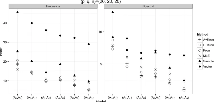
Figure 1. Heat maps of the three matrices used for simulation when p=20. The figure for Case3is random realization of the matrix generating process. Black color denotes 1 and white color denotes 0.
a sample sizen=20 and various dimensions as(p, q)=(20,20),(320,320)or(640,20). For each setup, we generate a test data with the same sample size and choose the tuning parameter that minimises the Frobenius norm of the difference between the estimate and the empirical covariance matrix of the test data.
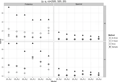
We first examine the estimation accuracy in the Frobenius and spectral norm respectively be-tween the truth and an estimator. The performance of various estimators of when (p, q)= (20,20)is presented in Figure2. Whenpqis large, computing the sparse vectorized estimator or a spectral norm is very slow. Thus, we only present the accuracy of estimating and for (p, q)=(320,320)in Figure 3 and for (p, q)=(640,20)in Figure 4 respectively. Here the maximum likelihood estimator is obtained via the flip-flop algorithm in Srivastava, von Rosen and von Rosen [18] which fails to give convergent solutions if n <min{p/q, q/p} +1 when
[image:12.488.44.421.354.534.2]Figure 3. The accuracy when(p, q, n)=(320,320,20). Short notations can be found in the caption of Figure2.
(p, q)=(640,20). This phenomenon happens because during the iteration, some of the esti-mated intermediate matrices are degenerate and thus cannot be used for updating. Finally, we also note that the naive sample estimator˜nis outperformed by all the estimators in Figure2by
a large magnitude (not shown) and thus is omitted for better visualization.
We can draw the following conclusions from these figures. The sample estimator and the sparse vectorized estimator are outperformed by the Kronecker estimators. The maximum likelihood estimator works well when(p, q)=(20,20), but loses out when dimensionality becomes large. Among the Kronecker estimators, the hard-thresholding estimator and the adaptive Kronecker estimator perform among the best, followed by the Kronecker estimator overall.
For variable selection, we follow Leng and Tang [13] to record the true positive rate defined as #{ ˆAij=0&Aij=0}/#{Aij=0}and the true negative rate defined as #{ ˆAij=0&Aij=0}/
#{Aij=0}. From Table1, we can see that the Kronecker estimators perform satisfactorily in
general, especially so for the hard-thresholding and adaptive estimators.
An interesting question arises regarding how robust the method is if the assumed Kronecker structure is not true. Towards this end, we generate data by assuming
Figure 4. The accuracy when(p, q, n)=(640,20,20). Short notations can be found in the caption of Figure2.
where and are specified as previously,I is anpq×pq dimensional identity matrix and α∈ [0,1]is a constant. Apparently, wheneverα∈(0,1), the assumed Kronecker structure does not hold. We find that under this perturbation scheme, the proposed method continues to perform better than the sparse vectorized estimator, an example of which withα=0.5 is illustrated in Figure5. This is most likely due to the reduction of the large number of parameters, the simple structure ofand the small sample sizen=20. We have also conducted additional simulations by assuming=Ai,i=1,2,3 which does not admit the Kronecker structure. We have observed
that the proposed methods continue to outperform the sparse vectorized estimator.
4.1. A data analysis
Table 1. Model selection result in percentages. TPR, true positive rate; TNR, true negative rate; Kron, Kronecker estimator; A-Kron, adaptive Kronecker estimator; H-Kron, Kronecker estimator via hard-thresholding
(p, q, n)=(320,320,20) (p, q, n)=(640,20,20)
(, ) Matrix Kron A-Kron H-Kron Kron A-Kron H-Kron
(A1, A1) TPR 100 100 100 100 100 100
TNR 92 99 100 42 93 98
TPR 100 100 100 92 88 78
TNR 92 99 100 94 99 100
(A2, A1) TPR 100 100 100 100 100 100
TNR 91 99 100 39 95 97
TPR 100 100 100 100 99 92
TNR 92 99 100 95 99 100
(A2, A2) TPR 100 100 100 100 100 100
TNR 91 100 100 51 99 100
TPR 100 100 100 100 100 99
TNR 91 100 100 95 99 100
(A3, A1) TPR 100 100 100 100 100 100
TNR 85 100 100 45 96 99
TPR 100 99 91 2 2 2
TNR 81 90 81 99 100 100
(A3, A2) TPR 100 100 100 100 100 100
TNR 91 100 100 50 99 100
TPR 100 100 99 7 2 2
TNR 75 93 100 99 100 100
(A3, A3) TPR 100 100 100 100 100 100
TNR 84 97 84 75 100 100
TPR 100 100 100 17 5 2
TNR 84 97 100 97 99 100
Figure 5. The accuracy when(p, q, n)=(20,20,20)when the true covariate matrix does not admit the Kronecker structure. Short notations can be found in the caption of Figure2.
To explore the covariance structure of the data, we start by vectorizing the matrices as vectors each with a dimensionpq=8584. We fit the penalized Gaussian graphical model in Yuan and Lin [23] for estimating a sparse−1and the sparse correlation matrix estimation method in Cui, Leng and Sun [8] for estimating a sparse . Using 10-fold cross validation for choosing their respective tuning parameter, both method estimateas a diagonal matrix. A formal test that the(pq)×(pq)dimensional correlation matrix is an identity matrix is rejected (Chen, Zhang and Zhong [7]). We proceed to use the sparse matrix variate graphical model in Leng and Tang [13] to estimatewhose inverse is represented as the Kronecker product of a sparse−1and −1. The tuning parameter is again chosen by 10-fold cross validation and we found that both matrices are estimated as diagonal.
Figure 6. The sampleandand their estimators based on the method in this paper. The sparsity is the percentage of the zeros in the corresponding matrix.
Finally, our Kronecker estimators from panels (c) and (f) confirm that a banded structure for the covariance matrix of the observed BOLD signals over the temporal domain might be appropri-ate.
5. Conclusion
Appendix A
We state a roadmap of the proof to Theorem1, consisting of two steps.
1. We first establish the following two bounds
tr1n−
max ≤C logq np and
tr1n−
max ≤C logp
nq , (6)
with certain probabilities. Moderate deviation for martingale is employed to establish (6) under the moment condition. To this end, a key step is to construct a martingale by ap-propriately rewriting the entry of the random matrix of interest. Once this is done, the next difficulty is to characterize the difference between the conditional variance and the variance of the martingale, which is accomplished by evaluating its higher moment.
2. We further derive the convergence rate of the correlation matrices by putting the correlation matrices into (3) and (4) in the main paper. Specifically, we obtain the convergence rate of (R−R)and(R−R)under the spectral norm and the Frobenius norm, respectively. To prove (6), we first write the expression of the elements of the matrices in (6) as
n p − tr() p max = max
u,v≤q
1 n n
k=1
1 p
p
i=1
(xk,iuxk,iv−ψuvσii)
, n q − tr() q max = max
u,v≤p
1 n n
k=1
1 q
q
j=1
(xk,ujxk,vj−ψjjσuv)
.
(7)
We then prove (6) by considering the(u, v)th element of the above matrices as independent sums or martingales.
For ease reference, we cite a moderate deviation result for martingales in Grama [9].
Lemma 1. Letznbe a martingale difference sequence with respect to the increasingσ-fieldFn.
Suppose that for someδ >0
Ln2δ=E
n
i=1
|zi|2+2δ→0, N2nδ=E
n
i=1
Ez2i|Fi−1
−1
1+δ
→0.
Suppose thatx is such that1≤x≤α(Ln2δ+N2nδ)−1withα >0.Then
P n
i=1
zi
≥r
=21−(r)1+θ C(α, δ)x3+12δLn
2δ+N n
2δ
1 3+2δ,
where|θ| ≤1,C(α, δ)is a constant depending only onαandδand
r2=2 logx−θ12c(δ)log(1+
2 logx),
Applying this lemma, we establish the following result whose proof can be found in supple-mentary materials.
Lemma 2. Assume that Conditions(A),(B)and(C)are satisfied.Then for someM >0,
Pn tr−
max
≤ p tr
Mlogq np
≥1−q−0.94,
Pn tr −
max
≤ q tr
Mlogp nq
≥1−p−0.94.
Proof of Lemma2. Throughout the paper, we useC andCj to denote constants which may
change from line to line.
We only prove the second inequality and the first one can be proved similarly. Define
Qquv=√nq
n
q − tr()
q
uv
.
By (7), write
Qquv=
1 √nq
n
k=1
q
j=1
(xk,ujxk,vj−ψjjσuv)
=√1nq
q
j=1
n
k=1
(xk,ujxk,vj−ψjjσuv)
. (8)
In order to decomposeQnuv into a sum of some manageable terms, we introduce the following
notation. Let
A=(aij)q×q=(a1, . . . , aq)T, ai=(ai1, . . . , aiq)T, i=1, . . . , q,
B=(bij)p×p=(b1, . . . , bp)T, bi=(bi1, . . . , bip)T, i=1, . . . , p,
Sk=(sk,ij)p×q=(sk,1, . . . , sk,q), sk,=(sk,1, . . . , sk,p)T, =1, . . . , q.
Recalling (1) in the main paper and the covariance matrices=AAT,=BBT, we have
φij=aiTaj, i, j≤q, σij=biTbj, i, j≤p,
xk,ij=biTSkaj= q
=1
aj bTisk,.
(9)
Denote the(i, j )entry ofATAbyφij=qk=1akiakj.
Using (8) and (9) and the fact that trATA=trAAT, we haveQ
quv=
q
=1J, where
J=
1
√nq
α<
φα(J1α+J2α)+
1
with J1α =
n
k=1bTusk,sk,αT bv, J2α =
n
k=1bTusk,αsk,T bv and J3 =
n
k=1(bTusk,sk,T bv −
bTubv). Define theσ fieldsF=σ (skm,k=1, . . . , n,m=1, . . . , ). Then one may verify that
E(J|F−1)=0. Furthermore a direct calculation indicates thatE|
q
J|< (Var(
q
J))1/2<
∞, as (10) below shows. Therefore,{J,F}is a sequence of martingale differences.
We next calculate the variance ofQquv. One may verify that
E
α<
φαJ1α
2
=E
α<
φαJ2α
2
=nbTububTvbv
α<
φα2
and
E
α1<
φα1J1α1
α2<
φα2J2α2
=nbuTbv
2
α<
φα2 .
It follows that the variance ofQquvis
Var(Qquv)= q
=1
Var(J)=
1 nq q =1 E α<
φα(J1α+J2α)
2 + 1 nq q =1
φ2E(J3)2
=bTububTvbv+(bTubv)2
q
q
=α
φα2
+1 q
q
=1
φ2
Es14,11−3
p
i=1
b2uib2vi+buTbubTvbv+
bTubv
2
.
Therefore
Var(Qquv)
2F
q , (10)
whereanbnmeans that there exist constantsc1andc2such thatc1an≤bn≤c2anasn→ ∞.
We now investigate N2nδ in Lemma1. To this end, we first evaluate the terms involved in E(J2|F−1). Note that
E(φJ3)2|F−1
=E(φJ3)2,
E
α<
φαJ1α×φJ3
F−1
=φ α< φα n
k=1
sk,αT bv
p
i=1
b2uibviEs13,11,
E
α<
φαJ2α×φJ3
F−1
=φ α< φα n
k=1
buTsk,α
p
i=1
b2vibuiEs13,11,
E
α1<
φα1J1α1
α2<
φα2J2α2
F−1
=
α1<,α2<
φα1φα2
n
k=1
sk,αT
1bvb
T usk,α2
E
α<
φαJ1α
2
F−1
=buTbu n
k=1
α<
φαsk,αT bv
2
,
E
α<
φαJ2α
2
F−1
=bvTbv n
k=1
α<
φαbuTsk,α
2
.
It follows that
q
EJ2|F−1
= 1 nq q E α<
φα(J1α+J2α)+φJ3
2
F−1
= 1 nq q E α<
φα(J1α+J2α)2F−1
+E(φJ3)2|F−1
+2E
α<
φα(J1α+J2α)φJ3F−1
= 1 nq q
buTbu n
k=1
α<
φαsk,αT bv
2
+bTvbv n
k=1
α<
φαbTusk,α
2
+2
α1<,α2<
φα1φα2
n
k=1
sk,αT
1bvb
T usk,α2
buTbv+E(φJ3)2
+Qn8+Qn9,
where
Qn8=2Es31,11
1 nq q φ α< φα n
k=1
sk,αT bv
p
i=1
b2uibvi
, (11)
and
Qn9=2Es13,11
1 nq q φ α< φα n
k=1
bTusk,α
p
i=1
bvi2bui
. (12)
We conclude from (10) and (11) that
q
EJ2|F−1
−Var q J
where
Qn1=bTubu
1 nq q n
k=1
α<
φ2αsTk,αbv
2
−bTvbv
q q α<
φα2
, (13)
Qn2=
2buTbu
nq q n
k=1
α1<α2<
φα1φα2s
T
k,α1bvs
T
k,α2bv,
Qn3=bTvbv
1 nq q n
k=1
α<
φα2 bTusk,α
2
−buTbu
q q α<
φα2
,
Qn4=
2bvTbv
nq q n
k=1
α1<α2<
φα1φα2b
T
usk,α1b
T
usk,α2,
Qn5=2buTbv
1 nq q n
k=1
α<
φα2 sk,αT bvbuTsk,α
−bTubv
1 q q q α<
φ2α
,
Qn6=2buTbv
1 nq q
α1<α2<
φα1φα2
n
k=1
sTk,α
1bvb
T usk,α2
and
Qn7=2bTubv
1 nq q
α2<α1<
φα1φα2
n
k=1
sk,αT
1bvb
T usk,α2
. (14)
In order to offset p2 caused by max in the inequality (17), below we evaluate the higher moments ofQnj,j=1, . . . ,9 in Lemma3below. By (10) and Lemma3we obtain
E
q
E(J2|F−1)
Var(qJ)
−1
12
≤Cq201( 0 1)
T12
F
n624
F
+ Cq6 n624
F
+C01( 0 1)
T6
F
n612
F
≤ C
n6q3,
(15)
where we use Lemma 2.1 of Bhansali, Giraitis and Kokoszka [2].
We next considerLn2δwithδ=11 in condition (1). By Rosenthal’s inequality
E(J)24≤
C
n12q12E
α<
φα(J1α+J2α)
24
+ C
n12q12φ 24
EJ
24 3 ≤
C
q12
α<
φα2
12
.
This, together with (10), yields that
1 (Var(qJ))12
q
=1
E(J)24≤
C
q11, (16)
From (15) and (16), we see thatCq3≤α(Ln2δ+N2nδ)−1with some appropriateC, independent ofq. Therefore choosexto beCq3in Lemma1. Note that Var(q=1J)≤Cby (10). It follows
from Lemma1that
P
max
u,v≤p
q =1 J ≥M logp
≤p2P
q =1J
Var(q=1J)
≥CMlogp
≤p2P
q =1J
Var(q=1J)
≥2tlogq3
≤ C
p3t−2,
(17)
whereMis chosen so thatCM√logp >2tlogq3with 2<3t <3. Selectingtso that 3t−2=
0.95 and then summarizing the above, the proof is complete.
Lemma 3. Recall the definitions ofQnj,j=1, . . . ,9in(11)–(14).Then
E(Qn1)12+ · · · +E(Qn9)12≤
C01(01)T12
F
n6q10 +
C n6q6+
C12F01(01)T6
F
n6q12 ,
where01=(φα0 )stands for the matrix obtained fromATA=(φ
α)withφα0 =φαifα < and
zero otherwise.
Proof of Lemma3. Note that the termsQn2,Qn4,Qn6andQn7are similar (their upper bounds
are the same up to the constants involvingbuTbv,bTubu,bTvbv). Therefore we only estimateQn2
below. Define
uα1α2=
>α2
φα1φα2, vα1α3=
α2>max(α1,α3)
uα1α2uα3α2.
Write
Qn2=
2 nq
n
k=1
α1<α2
uα1α2s
T
k,α1bvs
T
k,α2bv. By Rosenthal’s inequality,
E(Qn2)12≤
C n12q12
n
k=1
E
α2
α1<α2
uα1α2s
T
k,α1bvs
T
k,α2bv
2
6
+ C
n12q12
n
k=1
E
α2
α1<α2
uα1α2s
T
k,α1bvs
T
k,α2bv
12
≤ C
n6q12
α2
α1<α2
u2α
1α2
6+ C
n12q12
n
k=1
E
α2 α1<α2
uα1α2s
T
k,α1bv
+ C n12q12
n
k=1
α2
E
α1<α2
uα1α2s
T
k,α1bv
12
≤ C
n6q12 0 1
01T 12F + C n12q12
n
k=1
E
α1,α3
vα1α3s
T
k,α1bvs
T
k,α3bv
6
+ C
n12q12
n
k=1
α2 α1<α2
Euα1α2s
T
k,α1bv
26
+ C
n12q12
n
k=1
α2
α1<α2
Euα1α2s
T
k,α1bv
12
≤ C
n6q12 0 1
01T 12
F +
C n12q12
n
k=1
E
α3 α1<α3
vα1α3s
T
k,α1bv
23
+ C
n12q12
n
k=1
α3
E
α1<α3
vα1α3s
T
k,α1bv
6
+ C
n11q12
α2 α1<α2
u2α
1α2
6
≤ C
n6q12 0 1
01T 12
F +
C n12q10
n
k=1
α3
E
α1<α3
vα1α3s
T
k,α1bv
6
+ C
n11q12
α2
α1<α2
u2α
1α2
6
≤ C
n6q12 0 1
01T 12F + C n11q10
α3 α1<α3
vα2
1α3
3
+ C
n11q10
α3
α1<α3
v6α
1α3
≤ C
n6q12 0 1
01T 12
F +
C n11q10
α3
α1<α3
vα2
1α3
3
≤ C
n6q12 0 1
01T 12F + C n11q10
α3
α1<α3
α2>α1
u2α
1α2
α2>α3
u2α
3α2
3
≤ C
n6q10 0 1
01T 12
F,
where the third step uses the fact that
α2 α1<α2
uα1α2s
T
k,α1bv
2
=
α1,α3
vα1α3s
T
k,α1bvs
T
and the fact that
α2
α1<α2
u2α
1α2 =
1,2
α1<α2<min(1,2)
φ1α1φ1α2φ2α1φ2α2≤ 0 1
01T 2F,
and the step next to the last one uses Cauchy’s inequality.
Since the terms Qn1,Qn3 andQn5 are similar (their upper bounds are the same up to the
constants involvingbTubv,bTubu,bTvbv) we only considerQn1next. Letvα=
>αφα2 . Write
Qn1=
1 nq
n
k=1
α
vα
sk,αT bv
2
−bTvbv
q
α
vα.
It follows that
E|Qn1|12≤
C
n12q12
n
k=1
E
α
vα
sk,αT bvbTvsk,α−bvTbv
26
+ C
n12q12
n
k=1
E
α
vα
sk,αT bvbTvsk,α−bTvbv
12
≤ C
n12q12
n
k=1
α
vα2
6
+ C
n12q12
n
k=1
α
vα12≤ C n6q12
α
v2α
6
≤ C
n6q6,
where we use the fact thatvαis bounded.
We next consider Qn8 only since Qn8 and Qn9 are similar (see (11) and (12)). Note that
|p
i=1b2uibvi|is bounded. Defineuα=
>α(φφα). RewriteQn8as
Qn8=
2Es13,11 nq
n
k=1
α
sk,αT bvuα p
i=1
b2uibvi.
By Rosenthal’s inequality
E|Qn8|12≤
C n12q12
n
k=1
α
bTvbvu2α
6
+ C
n12q12
n
k=1
E α
sk,αT bvuα
12
≤ C
n6q12
α
u2α
6
+ C
n12q12
n
k=1
α
vTvbvu2α
6+ C n12q12
n
k=1
α
Esk,αT bv
12
u12α
≤ C
n6q12
α
u2α
6
+ C
n11q12
α
u2α
6
+ C
n11q12
α
u12α
≤ C
n6q12
α
u2α
6 ≤C 12 F 0 1( 0 1)T
6
F
because
α
u2α=
1,2
α<min(1,2)
φ11φ1α1φ22φ2α2
≤
φ2
1,2
α<min(1,2)
φ1αφ2α
21/2≤C2F 0101T F.
Appendix B
The aim of this section is to prove Theorem1, Corollary 1and Corollary 2. To simplify the presentation, we define the following two events,
X=
tr1n−
max
≤C
logq np
, X=
tr1n−
max
≤C
logp nq
,
whereCis a constant which may have different values in different places. By Lemma2we have the following Lemma.
Lemma 4. Assume that Conditions(A),(B)and(C)are satisfied.We have
P (X)=1−q−0.94, P (X)=1−p−0.94.
In the following, to ease the presentation, we assume that the two eventsX andXhold.
We next derive the convergence rate regarding the correlation matricesRnandRn.
Lemma 5. Assume that the eventsXandXhappen.We have
Rn−Rmax≤C
logq
np , R
n −R
max≤C
logp nq ,
whereC is a positive constant.
Proof of Lemma 5. We only prove the first inequality while the second one can be simi-larly proved. RecallRn =(W1)−1n(W1)−1andR=(W)−1(W)−1, where(W)2=
diag(). When the eventXhappens, we have|tr1(W1)2ii−ψii| ≤C
logq
np for alli≤q. Then,
there exist positive constantscandCsuch that
c≤W1
ii/
√
tr≤C, √1 tr
W1
ii−
ψii
≤C