Performance evaluation of empirical models for vented lean hydrogen explosions

warwick.ac.uk/lib-publications

Manuscript version: Author’s Accepted Manuscript

The version presented in WRAP is the author’s accepted manuscript and may differ from the published version or Version of Record.

Persistent WRAP URL:

http://wrap.warwick.ac.uk/109492

How to cite:

Please refer to published version for the most recent bibliographic citation information. If a published version is known of, the repository item page linked to above, will contain details on accessing it.

Copyright and reuse:

The Warwick Research Archive Portal (WRAP) makes this work by researchers of the University of Warwick available open access under the following conditions.

© 2018 Elsevier. Licensed under the Creative Commons Attribution-NonCommercial-NoDerivatives 4.0 International http://creativecommons.org/licenses/by-nc-nd/4.0/.

Publisher’s statement:

Please refer to the repository item page, publisher’s statement section, for further information.

Performance Evaluation of Empirical Models

for Vented Lean Hydrogen Explosions

Anubhav Sinha, Vendra C. Madhav Rao, Jennifer X. Wen*

School of Engineering, University of Warwick,

Coventry CV4 7AL, UK

*Corresponding author: [email protected]

Abstract – This paper aims to provide a comprehensive review of available empirical models

for overpressures predictions of vented lean hydrogen explosions. Empirical models and standards are described briefly, with discussion on salient features of each model. Model predictions are then compared with the available experimental results on vented hydrogen explosions. First comparison is made for standards tests, with empty container and quiescent starting conditions. Comparisons are then made for realistic cases with obstacles and initial turbulent mixture. Recently, a large number of experiments are carried out with standard 20-foot container for the HySEA project. Results from these tests are also used for model comparison. Comments on accuracy of model predictions, their applicability and limitations are discussed.

A new model for vented hydrogen explosion is proposed. This model is based on external cloud formation, and explosion. Available experimental measurements of flame speed and vortex ring formation are used in formulation of this model. All assumptions and modelling procedure are explained in detail. The main advantage of this model is that it does not have any tuning parameter and the same set of equations is used for all conditions. Predictions using this model show a reasonably good match with experimental results.

Keywords – vented explosions, empirical model, new engineering model, deflagrations,

1. Introduction

Vented explosion is an important technique to relieve pressure in industrial enclosures and

low strength buildings. Vent panels are designed based on the allowable peak pressure inside

a building. To investigate peak overpressure attained in an accidental scenario, experiments

can be both expensive and time consuming, especially in case of larger enclosures.

Computational studies are also employed in these investigations, but studying a realistic size

enclosure involves prohibitively large computational costs. Moreover, due to the large range

of length and time scales involved in the phenomenon of vented explosion, accurately

predicting overpressures is a challenging task. Empirical engineering models provide a fast

and convenient method to predict overpressure, and can give an acceptable level of accuracy

without much effort. Previous studies on vented explosions have mostly focussed on

hydrocarbon gaseous fuels (Bauwens et al. [1]), dust, and vapours formed from liquid fuels.

Recently, there has been a surge in use of hydrogen as a clean fuel and installations using and

storing hydrogen are expected to increase in future. The objective of this paper is to present a

review of available empirical models for overpressure predictions for hydrogen explosions,

and provide recommendations of the suitability and applicability of them for various

conditions. Further, a new phenomenological model is also proposed to predict overpressures

in hydrogen deflagrations. Model formulations and major assumptions are explained in detail.

Various physical processes observed in vented deflagrations are accounted for and included

in the model formulation. Predictions from this new model are found to be in good agreement

with the available experimental results. The model does not involve any tuneable constants or

adjustable parameters and predictions are made following the same set of equations for all

cases.

Section 2 begins with a brief description of empirical models and major assumptions used in

them. Section 3 shows the comparison of model predictions with experimental measurements.

Section 4 gives formulation for a new model and explain its formulations and equations to be

used. Predictions from this model are also compared with the experimental results and found

2. Empirical Models for Overpressure Predictions

Four models are discussed in this section. They include the statutory standards – (i)

EN-14994 [2], (ii) NFPA-68 [3], and other empirical models (iii) FM Global model [1, 4-6], and

(iv) Molkov model [13].

2.1. EN-14994 Model [2] – The EN-14994 model is a part of statutory norms across Europe.

The latest version available for this model was published in 2007 [2]. This model is based on

gas explosion constant KG. KG is defined as the maximum value of pressure rise per unit time

in a standard vessel. It is to be noted that this vessel is closed from all sides and different

from the vented enclosure environment where this model is applied. One of the objectives of

defining KG for a closed vessel is that it can be measured with good repeatability and for

different gases by maintaining the standard conditions. This model is divided into three

formulations – (i) for compact enclosures (L/D<2), (ii) Elongated enclosures (2≤ L/D ≤ 10),

(iii) pipe (L/D > 10). First two formulations which are applicable for enclosures are discussed

here.

(i) Compact Enclosure – The vent area for a given maximum pressure can be calculated

using the following equation:

𝐴_𝑣 𝐸_𝑓 = [{(0.1265 ln(𝐾_𝐺) − 0.0567)𝑝−0.5817_{} + {0.1754𝑝}−0.5722_(𝑝

𝑠𝑡𝑎𝑡 − 0.1 𝑏𝑎𝑟)}]𝑉2/3

(2.1)

where 𝐴_𝑣is the vent area of enclosure, 𝐸_𝑓 is the venting efficiency (𝐸_𝑓=1 is used for lighter

vents considered in this study), is the 𝑝 peak overpressure, 𝑝_{𝑠𝑡𝑎𝑡} is the static pressure, 𝑉 is

the volume of the enclosure. This equation is designed for calculating required venting area

for a known permissible overpressure. This equation can also be modified to calculate the

peak overpressure produced with a given vent area, as is done in the present study. This

formulation does not account for initial turbulence, presence of obstacles, stratified fuel

distribution, higher initial pressure, and partially filled enclosure. It is also recommended to

be used for mixtures with KG ≤ 550 bar ∙ m/s. KG values for hydrogen used in this study are

obtained from the experimental measurements of Holtappels et al. [33].

(ii) Elongated Enclosure – Three equations are proposed to calculate overpressure for this

𝑝 = 𝑝_{𝑠𝑡𝑎𝑡} +(0.023 ∙ 𝑆𝐿𝐾𝑊(𝐿 𝐷)⁄

1/3

𝑉1/3 (2.2)

𝑝 = 0.015 𝑑𝐾 (2.3)

𝑝 = 0.015 𝑑 ∙ 𝐾 + 0.15 (2.4)

where 𝑆𝐿is the laminar burning velocity, 𝐾 is the vent coefficient – ratio of vessel

cross-sectional area and total vent area, W is the weight per unit area of vent panel, 𝐷 is the enclosure diameter, 𝐿 is the enclosure length, 𝑑 can be defined as:

𝑑 = 𝑥/𝐷

where 𝑥 is the maximum possible distance between ignition location and vent area. The

parameters are to be specified in SI units. Equation 2.3 is to be used for 𝑝_{𝑠𝑡𝑎𝑡}≤ 0.06 bar and

equation 2.4 is to be used when 𝑝𝑠𝑡𝑎𝑡 > 0.06 bar.

2.2. NFPA-68 Model [3]– This model by National Fire Protection Association is the

American standard model. The latest version available was published in 2013 [3]. The

formulation recommends two different methods to be used (i) for reduced overpressure ≤ 0.5

bar, (ii) for reduced overpressure > 0.5 bar.

(i) For 𝒑 ≤ 0.5 bar - The recommended minimum vent area can be calculated for cases with

p ≤ 0.5 bar by using:

𝐴𝑣 =

𝐴_𝑠 𝐶

√𝑝

where 𝐴𝑣 is the vent area, 𝐴𝑠 is the internal surface area of enclosure, 𝑝 is the reduced

overpressure, and parameter 𝐶 can be estimated as:

𝐶 = 𝑆𝐿 𝜆 𝜌𝑢 2 𝐺_𝑢 𝐶_𝑑[(

𝑃_𝑚𝑎𝑥 + 1 𝑃₀+ 1 )

1/𝛾𝑏

− 1] (𝑃₀+ 1)1/2 (2.5)

where 𝑆_𝐿 is the burning velocity of the mixture, 𝜆 is a factor that accounts for turbulence and

vent, 𝐺_𝑢 is the unburnt mixture sonic flow mass flux (𝐺_𝑢=230.1 kg/m2-s for an initial temp of

200 C), 𝑃𝑚𝑎𝑥 is the maximum pressure that can develop in the enclosure by burning the

same gas mixture, 𝑃₀ is the initial static pressure, 𝛾_𝑏 is the ratio of specific heat of the burnt

gases.

(ii) For 𝒑 > 0.5 bar - The formulation for higher static pressure can be given as:

𝐴𝑣 = 𝐴𝑠

[

1 − (_𝑃𝑃 + 1

𝑚𝑎𝑥 + 1) 1/𝛾𝑏

(_𝑃𝑃 + 1

𝑚𝑎𝑥 + 1) 1/𝛾𝑏

− 𝛿_] 𝑆_𝐿 𝜌_𝑢

𝐺𝑢

𝜆 𝐶𝑑

(2.6)

Where 𝛿 can be defined as:

𝛿 =

(𝑃𝑠𝑡𝑎𝑡_𝑃 + 1

0+ 1 )

1/𝛾𝑏

− 1

(𝑃𝑚𝑎𝑥_𝑃 + 1

0+ 1 )

1/𝛾𝑏

− 1

To calculate the required vent area, it is required to guess a starting value of area, calculate

pressure from it, and then iterate until the guessed pressure matches with the allowed pressure.

This iterative procedure makes this model relatively difficult to use compared to other models.

2.3. FM Global model – The FM Global model [1, 4-6] is based on several experimental

studies on their 63.7 m3 enclosure, consisting of tests on hydrogen, methane and propane. The

same set of equations is applicable for all these gases. This model hypothesises that there are

three different factors responsible for pressure rise inside an enclosure – (i) External

explosion (P1), (ii) Flame-acoustic interaction (P2), (iii) Flame wrinkling caused by obstacles

(P3). These factors are responsible for multiple peaks observed in pressure transient

measurements. Peak pressures for these processes are calculated separately and the maximum

of these three peaks is the resultant overall peak overpressure. The model builds on the

theoretical derivations of [7, 8] which describe the flame propagation inside enclosure,

pressure rise due to volumetric expansion of burnt products and pressure loss due to venting.

The final overpressure depends on the interplay of these processes. Various physical

processes and fuel properties are considered. The equation to calculate overpressure is given

𝑝 𝑝e

= 𝑝e𝐺

𝐴_v∗ 2₊ 𝑝e2𝐺

(𝑝cv− 𝑝e)

+ 1 (2.7)

where 𝑝 is the pressure inside the enclosure, 𝑝_𝑒 is the external pressure, 𝑝_cv is the constant

volume explosion pressure, 𝐺 is given by:

𝐺 = (𝛾 + 1

2 )

𝛾 (𝛾−1)

− 1

and 𝐴v∗ can be calculated using:

𝐴_𝑣∗ ₌ 𝑎cd𝐴v

𝑆u𝐴f(𝜎 − 1)

(2.8)

where 𝑆_𝑢 is the flame speed, 𝐴_𝑓is the flame surface area, 𝜎 is the expansion ratio, 𝐴_𝑣is the

vent area, 𝑎_𝑐𝑑 is a parameter given as:

𝑎_𝑐𝑑= 𝑐_𝑑 √𝑅𝑇𝑣 𝑀_𝑣 𝛾

𝛾 + 1 2

where 𝑐𝑑 is the discharge coefficient (𝑐𝑑=0.61 is recommended), 𝑅 is the universal gas

constant, 𝑇_𝑣 and 𝑀_𝑣 are vented gas temperature and molecular weight respectively, and 𝛾 is

the ratio of specific heat capacities for the vented gases. It is assumed that the vented gases

consist 90% of burnt gases and 10% of unburnt gases, and vent gas properties are computed

using their weighted average. Flame area is calculated based on simplified geometric

assumptions. The flame-ball is assumed to be approximately spherical for central ignition and

half-ellipsoidal shaped for back-wall ignition. This formulation is used to calculate P1, the

pressure peak due to external cloud. External pressure 𝑝_eis given by

𝑝_e

𝑝₀− 1 =

5𝛾(𝜎 − 1)𝜎𝑟_e𝑆_u 𝐴𝑅 √𝑘_T𝑎

𝑢_s2 (2.9)

where 𝑝0is the ambient pressure, 𝑟eis the external cloud radius, 𝑢𝑠 is sonic speed in unburnt

A closer examination of equations 2.7 - 2.9 reveals the significance of each of the three

processes. A higher value of external explosion will have higher 𝑝_𝑒and hence it will become

dominant term for the overall peak pressure. Moreover, increase in burning velocity (𝑆𝑢) due

to flame-acoustic interaction is expected to give a higher peak pressure P2. Lastly, it is

understood that the obstacles increase the burning rate by increasing the flame surface area

(𝐴𝑓) by wrinkling. So a larger 𝐴𝑓 will result in the dominant contribution from the obstacles.

For estimating transient peak P2, the flame is assumed to approach the internal walls and 0.9

times the internal surface area is used as the flame surface area. The flame speed for acoustic

peak (P2), the laminar flame speed is multiplied by an acoustic coefficient whose value is

determined using best fit with the experimental data. The values used in the present study is

in the range 1.29 to 3.1 [11]. For increase in 𝐴𝑓 because of obstacles, a model by Dorofeev [9,

10] is employed. This gives the third pressure transient P3. The original formulation of this

model had some issues with containers having large L/D, but this issue has been addressed in

a recent update [11]. For the present study, fuel properties to be used for this model are

calculated using the GASEQ calculator [12]. For obtaining acoustic coefficient and kT , some

useful guidelines are also provided by Jallais and Kudriakov [34].

A simplified version of this model is also published recently [36]. It is based on worst

scenario approximation and is majorly based on this basic model. The final equation for

overpressure is simplified version of equation 2.7 and can be stated as:

𝑝 𝑝_e=

𝑝e𝐺

𝐴_v∗ 2 + 1

Other equations of the simplified model are mostly similar to the basic detailed model.

However, the detailed model is used for the present study.

2.4. Molkov and Bragin Model (2015) – This model [13] is based on a novel concept of

turbulent Bradley number, and it is based on previous versions of the same model and several

numerical studies by the author and his group on vented deflagrations [14-19]. Bradley

number can be defines as:

𝐵𝑟 = 𝐴𝑣

𝑉2/3

where 𝐴_𝑣 is the vent area, 𝑉 is the enclosure volume, 𝑐_𝑢 is the speed of sound in unburnt

gases, 𝑆𝐿 is the laminar burning velocity, and 𝜎 is the expansion ratio. This is further used to

define turbulent Bradley number:

𝐵𝑟𝑡=

√𝜎/𝛾

√36 𝜋0 3

𝐵𝑟 𝜒/𝜇

where 𝛾 is the specific heat ratio for unburnt gases, 𝜋₀= 3.141, (𝜒/𝜇) is the

deflagration-outflow interaction (DOI) number, in which is 𝜒 the turbulence factor and is the 𝜇 discharge

coefficient. The basic assumption of this model is that the turbulent Bradley number

correlates with overpressure. Various experimental studies are used to get curve-fit for this

correlation and two equations are proposed. First is the equation that gives the best-fit values

with the experimental data:

𝑝 = 0.33 𝐵𝑟_𝑡−1.3 _(2.10)

where 𝑝 is the reduced overpressure. The second equation is intended to give a conservative

estimate:

𝑝 = 0.86 𝐵𝑟_𝑡−1.3 _(2.11)

However, in this study, results using the best-fit model are only given. To calculate

overpressure using these equations, in addition to fuel properties, DOI number also needs to

be calculated. DOI number can be estimated by multiplying factors from various processes:

𝜒

𝜇= 𝛯𝐾 ∙ 𝛯𝐿𝑃∙ 𝛯𝐹𝑅 ∙ 𝛯𝑢′∙ 𝛯𝐴𝑅 ∙ 𝛯0 (2.12)

where 𝛯_𝐾 is the factor for turbulence generated by the flame-front, 𝛯_𝐿𝑃 is factor for leading

point, 𝛯𝐹𝑅 is the factor to account for the increase in flame-front area due to fractal nature of

flame surface, 𝛯_𝑢′is the factor to account for initial turbulence, 𝛯_𝐴𝑅is the factor for, 𝛯₀is the

factor to account for increased wrinkling due to presence of obstacles. No theoretical

foundation has been given for this formulation of the DOI number and it appears to be of

empirical nature. However the authors mention to have used computational modelling to

formulate this equation, no derivation or detailed explanation is available. They have,

however, given complete formulations to calculate all factors used in equation 2.2, except for

the factor for obstacles, 𝛯0. For this factor, lack of experimental data is cited as a reason and

calculated but suggested based on the best-fit obtained with the experimental results. As such

it becomes challenging to use this formulation for predictions of cases with obstacles. A

useful extension of this model is also proposed recently [37] which deals with the case of

3. Model Predictions for Overpressure

Overpressure predictions from the above discussed models are compared with available

experimental results. The experimental results used in this evaluation are from the studies of:

(i) Bauwens et al. [4]

(ii) Kumar [20]

(iii) Daubech et al. [21]

(iv) Kumar [22]

(v) Bauwens et al. [23]

(vi) Schiavetti and Carcassi [24]

(vii) Skjold et al. [25]

(viii) Daubech et al. [35]

The experimental results are divided into various sets depending upon the complexity of the

experiments and their applicability in real accidental scenarios.

3.1 Standard Experiments – These experiments are carried out in an empty enclosure, with

uniformly mixed fuel and quiescent initial mixture. These simplified experiments are

different from actual accidental scenarios but offer set of standard and simple experiments

which can be used to test the applicability of empirical models. The main objective in these

experiments is to characterize the effect of parametric variations of fuel composition, vent

area, and ignition location. The experiments considered under this section are –

(i) Bauwens et al. [4]

(ii) Kumar [20]

(iii) Daubech et al. [21]

Bauwens et al. [4] carried out experiments in their 63.7 m3 _{cuboidal enclosure and tested the}

variation of hydrogen concentrations, vent areas, and ignition locations. They have also used

obstacles to model realistic accidents. The cases with obstacles will be considered in section

3.3. Kumar [20] has used 120 m3 cuboidal enclosure, and studied the variation of vent size,

ignition location and hydrogen concentrations. Kumar [20] has used the largest enclosure

considered in this study and the experiments have used very lean mixtures of hydrogen (6% -

12%). Daubech et al. [21] have used two cylindrical enclosures of 1 m3 and 10 m3 volumes

and have studied the effect of variation of hydrogen concentration in both the enclosures.

Daubech et al. [35] also carried out experiments in a cuboidal 4 m3 enclosure with a

transparent front wall. They have visualized flame propagation and external cloud formation.

The comparison of model predictions and overpressure measurements for Bauwens et al. [4]

is shown in figure 1. Three ignition locations used are marked in the figure – central ignition

(C), back-wall ignition (BW) and forward –wall (FW) ignition. As observed, the EN-14994

and NFP-68 models are over-predicting the pressure for all data points. FM Global model and

Molkov model show reasonably good match. Molkov model is under-predicting for all

back-wall ignition cases and over-predicting for all forward-back-wall ignition cases. This can be

attributed to the model formulation, where ignition location is not accounted for. Figure 2

shows comparison of model predictions with measurements of Kumar [20]. Different data

points are marked for different ignition locations. Interestingly, EN-14994 model which

over-predicted all data points for Bauwens et al. [4] is under-predicting some data points. These

data points are for higher hydrogen concentrations. So, it can be inferred that EN-14994

model over-predicts for lower fuel concentrations and under-predicts for higher fuel

concentrations. NFPA-68 is consistent with the trend shown in the previous example and is

also over-predicting for all data points. FM Global model show significant under-predictions

for many data points, and except for a few points, all other points are under-predicted.

Molkov model shows a large scatter, but shows a reasonable accuracy for many data points.

It is to be noted that this data set is for very low hydrogen concentrations (6% - 12%), and

enclosure with high L/D [20]. Hence, it can be inferred that the Molkov model is most

(a) EN-14994 Model (b) NFPA-68 Model

(c) FM Global Model (d) Molkov Model

(a) EN-14994 Model (b) NFPA-68 Model

(c) FM Global Model (d) Molkov Model

Figure 2. Model predictions for experiments of Kumar [20] compared with experimental results

Figure 3 shows comparison of model predictions with measurements of Daubech et al. [21].

The experiments are carried out at cylindrical enclosures with high L/D ratio. Data from

different enclosures are shown in different symbols. The EN-14994 model over-predicts for

lower hydrogen concentrations and under-predicts for higher hydrogen concentrations

(around 20% and above). NFPA-68 over-predicts for most data points, but is seen to

under-predict for hydrogen concentration of 10% to 20% in both the enclosures. Similar trend is

shown by FM Global model which under-predicts for approximately same fuel

shows reasonable accuracy, and most of the predictions are close to experimental

measurements.

(a) EN-14994 Model (b) NFPA-68 Model

(c) FM Global Model (d) Molkov Model

Figure 3. Model predictions for experiments of Daubech et al. [21] compared with experimental results

(a) EN-14994 Model (b) NFPA-68 Model

(c) FM Global Model (d) Molkov Model

Figure 4. Model predictions for experiments of Daubech et al. [35] compared with experimental results

3.2. Presence of initial turbulence – In this section, cases where turbulence is generated in

the unburnt mixture are considered. In an actual installation, accidents are caused by leaking

accidental scenario as compared to cases considered in previous section (3.1). Two studies

considered here are –

(i) Kumar [22]

(ii) Bauwens et al. [23]

These investigations are carried on the same 120 m3 (Kumar [22]) and 63.7 m3 (Bauwens et

al. [23]) enclosures used in previous studies discussed in section 3.1. The only difference is

that in these set of experiments, fans are installed inside the enclosures and the initial flow

field is made turbulent before the mixture is ignited. The turbulent fluctuations (u’) are measured to be 1 m/s for Kumar’s [22] study, while for Bauwens tests [22] u’ vary from 0.09 m/s to 0.5 m/s for various experiments. EN-14994 and NFPA-68 models do not account for

initial turbulence and hence only FM Global and Molkov’s model will be used in subsequent

discussion.

Figure 5 shows the comparison of results from Kumar [22] with predictions from FM Global

model and Molkov model. Kumar [22] has used different vent areas which are shown by

different symbols. It is observed that both these models are under-predicting for almost all

conditions. However, the predictions are in reasonable agreement with the measurements.

Molkov model is observed to give slightly more accurate results than the FM Global model.

Figure 6 shows comparison for data from Bauwens et al. [23] with predictions from these

models. It can be seen that the FM Global model shows a good agreement, while the Molkov

model shows several over-predictions for all data points. It seems that the FM Global model

(a) FM Global Model (b) Molkov Model

Figure 5. Model predictions for experiments of Kumar [22] compared with experimental results

(a) FM Global Model (b) Molkov Model

Figure 6. Model predictions for experiments of Bauwens et al. [23] compared with experimental results

3.3. Presence of Obstacles – In actual installations, the enclosures and buildings are

flame-path. Hence these cases represent accidental scenario more closely. Experimental

studies considered in this section are:

(i) Bauwens et al. [4]

(ii) Schiavetti and Carcassi [24]

(iii) Skjold et al. [25]

Figure 7 shows predictions for results from Bauwens et al. [4] containing obstacles. Both the

ignition locations used in experiments are shown with different symbols. As evident, both the

models are giving reasonably accurate predictions. It is to be noted that while the FM Global

model provide a complete formulation to account for obstacles, Molkov model provides a

tuneable constant (𝛯₀), whose best-fit value has to be used. Values of 𝛯₀ used here are 3.5 for

back-wall ignition and 1 for central ignition case. A modification of Molkov model to include

proper formulation of this constant will make this model very useful for practical accidental

scenarios.

(c) FM Global Model (d) Molkov Model

Figure 7. Model predictions for experiments of Bauwens et al. [4] with obstacles compared with experimental results

Schiavetti and Carcassi [24] carried out a systematic study to assess the effect of different

predictions are shown in figure 8. 𝛯₀ = 2 is used in Molkov model for all data points shown

in figure 8. Both the models show large scatter in predictions. Generally, for experiments

with obstacles, standard cylinders with circular or square cross sections are used. For these

experiments Schiavetti and Carcassi [24] have used flat plates which have different

recirculation regions than the standard cylinders. This different behaviour of flat plates can

possibly be related to the large scatter in these predictions. It also highlights the fact that

fundamental physics of the flow field need to be accounted for to get reasonable predictions

in realistic accidental scenarios.

(c) FM Global Model (d) Molkov Model

Figure 8. Model predictions for experiments of Schiavetti and Carcassi [24] compared with experimental results

It is evident that most previous experimental investigations focussed on standard conditions

with empty enclosures and quiescent mixture. To address the need for studies focussing on

practical accidental conditions, recent experiments were conducted under the HySEA project.

Under this project Skjold et al. [25] have used 20-foot ISO containers and conducted several

experiments which mimic practical conditions with different model obstacles. They have also

shown that covering vent area using commercial vent panels instead of plastic sheet results in

slightly higher peak pressure values. They have used two configurations with the ISO

basket and pipe rack as obstacles. More details about the experimental configuration can be

found in [25, 32]. Figure 9 shows the predictions for cases with empty containers.

(a) FM Global model – no obstacles (b) Molkov model– no obstacles

Figure 9. Model predictions for experiments of Skjold et al. [25] compared with experimental results

As evident, FM Global model shows slight under-prediction for door vented cases, and minor

over-predictions for all roof-vented cases. Molkov model show similar scatter in roof-venting

cases. Interestingly, it shows over-predictions for most roof-vented cases using plastic cover,

while cases using commercial vent panel are under-predicted. Figure 10 show predictions for

cases with obstacles using FM Global model and Molkov model. A constant value of 𝛯₀=1.25

is used for both bottle basket and pipe rack in Molkov model. In case where both bottle

basket and pipe rack are used 𝛯0=2.5 is used. Figures 10(a) and 10(b) show cases with door

venting, and figures 10(c) and 10(d) show cases with roof venting. For door venting, almost

all cases are over-predicted by FM Global model. The Molkov model shows good match at

lower over-pressures, but for higher overpressures Molkov model shows under-prediction.

Similarly, for roof venting, FM Global model shows over-prediction for all data points;

whereas Molkov model show under-prediction for most data points. It is to be noted that

previous experiments Bauwens et al. [3] and Schiavetti and Carcassi [24] have used standard

geometrical shapes as obstacles, whereas the HySEA experiments have used actual objects

appears that the realistic obstacles are more challenging to include in engineering model and

more experiments and modelling efforts are needed in this direction. In general, more

experimental results are needed for realistic conditions which include – presence of obstacles,

initial turbulence, stratified fuel distribution, multiple vents, etc.

(a) FM Global Model – door venting, (b) Molkov Model– door venting

(c) FM Global Model – roof venting (d) Molkov Model– roof venting

4. New Engineering Model

4.1. Modelling Details

As discussed in previous sections, and previous reviews [31], improvements in the existing

models or a new model are required to predict for more realistic scenarios. Physical processes

involved in vented explosions should be accounted in the modelling efforts. This will help in

modelling for new configurations and adding new features to the model, if required. The

present section presents the formulation of a new model which attempts to model different

physical processes in vented explosions. The vented deflagration phenomenon can be divided

into several physical processes, which can be listed as:

(i) Ignition and spherical flame propagation

(ii) Venting of unburnt mixture and formation of the external cloud

(iii) Combustion of the external cloud producing external pressure

(iv) Internal flame generating overpressure

These processes can be modelled separately based on the underlying physical phenomenon,

then the combinations of these sub-models can be used to compute the peak overpressure.

The main advantage of formulating such a modular framework is that new features, like

sub-models for obstacles and stratification can be added to the basic framework at a later stage

without modifying other sub-models. Also, improvements in a particular part can be made

without altering other sub-models. The modelling process can be explained in details as

follows:

(i) Ignition and spherical flame propagation - The spherical flame propagation for

hydrogen has been studied by several researchers. Recently, in a detailed study, Bauwens et

al. [26] measured the spherical flame propagation in a 63.7 m3 _{chamber and presented}

variation of flame propagation speed with radius using Background Oriented Schlieren (BOS)

technique for various hydrogen concentrations. The results of this study will be used to model

flame propagation. The flame propagation velocity with radius can be written as:

𝑈 𝑈0

= (𝑅 𝑅0

)

𝛽

where 𝑈 is the flame propagation velocity at radius 𝑅, 𝑈₀ is the flame propagation velocity at

𝑅0, which is the critical radius for the onset of cellular instabilities, and 𝛽 is fractal excess,

experimentally observed to be constant at 0.243 for all hydrogen concentrations [26]. The

values of 𝑈0and 𝑅0can be calculated using curve-fits to the experimental data [11, 26]

𝑈0 = 0.0537 x2− 1.008 x + 5.5716

𝑅₀ = (1.4273 x − 0.1942)/1000

where x is the hydrogen concentration in percentage. Since:

𝑈 = 𝑑𝑅

𝑑𝑡

Hence,

𝑑𝑅

𝑑𝑡 = 𝑈0( 𝑅 𝑅0

)

𝛽

.

Rearranging and integrating

∫ 𝑑𝑅

𝑅𝛽 𝑅

0

= ∫ 𝑈0

𝑅₀𝛽

𝜏

0

𝑑𝑡

𝑅(1−𝛽)

1 − 𝛽 = (

𝑈₀

𝑅₀𝛽) 𝜏 (4.2)

where, 𝜏 is the time taken by the flame to reach the radial position of R. This equation can be used to calculate the time for the flame-front to reach the vent. The distance from the ignition

source to the vent (R) can be estimated as:

𝑅 = {

𝐿 for Back − wall ignition 𝐿

2 for Central − ignition

where L is the length of the enclosure. So, for a known L, time taken can be calculated as:

𝜏 = (𝑅

(1−𝛽)

1 − 𝛽) ( 𝑅0𝛽

𝑈₀ ) (4.3)

(ii) Venting of unburnt mixture and formation of the external cloud- To study the

external cloud, it is assumed that the enclosure acts like a piston-cylinder arrangement, where

the flame-front pushing the gases work like a piston. The formation of external cloud by these

vented gases is then calculated using the vortex ring theory given by Sullivan et al. [27]. The

objective is to calculate the radius of the external cloud. To calculate the volume of the

vented gases forming the cloud, the volume of the flame-ball inside the enclosure is required.

Some simplifying assumptions for the flame shape are taken as: the flame-ball is considered

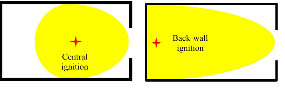
to be a half ellipsoid for a Back wall ignition case and a sphere for a Central ignition case.

The flame shape is shown in a schematic in Fig. 11.

(a) Central ignition (CI) (b) Back-wall ignition (BWI)

Figure 11. Schematic of the flame-shapes for different ignition locations

The flame-ball volume for the Central-ignition case can be calculated as:

𝑉_𝑏 = (4 3𝜋𝑅𝑒𝑞

3_{) (4.4)}

where 𝑅𝑒𝑞3 is the radius of the equivalent sphere.

𝑅_𝑒𝑞 =𝐵 + 𝐻 4

while for the Back-wall ignition case, the burnt volume can be estimated by calculating the

volume of the semi-ellipsoid

𝑉_𝑏= 𝜋

6𝐿𝐵𝐻 (4.5)

Central

ignition

Where L, B and H are the length, breadth and height of the enclosure, respectively. Finally, for both the cases, the volume of cloud can be calculated as:

𝑉𝑐 = 𝑉𝑏(1 −

1

𝜎) (4.6)

where 𝑉𝑐 is the cloud volume, 𝜎 is the gas expansion ratio. Now, for the piston, the

equivalent radius (R₀) can be calculated by equating the piston surface area to the vent area

(A_v)

𝑅0 = √

𝐴_𝑣 𝜋

Piston stroke length using the cloud volume and equivalent piston area:

𝐿_𝑃 = 𝑉𝐶 𝐴_𝑉

Saffman Vortex core size [27]:

𝑎 = √4 𝜈 𝜏

Radius of the vortex ring:

𝑅𝑅𝑖𝑛𝑔 = √

3 𝑅₀2 𝐿 4𝛼

3

where, 𝛼 = 1

Ʌ = ln (8𝑅𝑅𝑖𝑛𝑔

𝑎 ) − 0.558

k=0.65, and

𝑅_𝑏 = √ 9 𝜋 𝑅0

2 _𝐿 𝑃

4𝛼2_{Ʌ (1 + 𝑘)} 3

(4.7)

Radius of the external cloud is calculated using equation 4.7. More details about the cloud

formation and comparison of experimentally measured cloud diameters and predictions from

Equation 4.7 can be found in [28]. The cloud radius is further used to calculate overpressure

(iii) Combustion of the external cloud and external pressure produced –For external

cloud combustion, the flame propagation velocity at cloud radius 𝑅_𝑏 can be obtained from

equation 1. For pressure calculation, assuming Taylor’s spherical piston theory [29], the

Mach number at the cloud radius can be calculated as:

𝑀_𝑃 = 𝑈𝑐𝑙𝑜𝑢𝑑

𝑎₀ (4.8)

where 𝑀𝑃 is the Mach number at the cloud boundary, 𝑈𝑐𝑙𝑜𝑢𝑑is the flame-speed at the cloud

boundary, which can be calculated using equation 4.1 and cloud radius, 𝑎₀is the speed of

sound in unburnt gas mixture. The external pressure generated by this external cloud

combustion can be estimated as:

𝑃_𝑒𝑥= 2 𝛾_𝑢(1 −1 𝜎) 𝜎

2 _𝑀

𝑃2 (4.9)

Where 𝛾𝑢 is the ratio of specific heat of unburnt gases, and 𝜎 is the expansion ratio. This

external pressure will be used for calculating pressure generated inside the enclosure, as

described in the next section.

(iv) Internal flame generating overpressure - The fire-ball produced inside the enclosure

can be approximated as standard geometrical shapes as explain in previous section. The flame

area for those shapes can be calculated as:

𝐴 (𝑠𝑝ℎ𝑒𝑟𝑒) = 4𝜋𝑅𝑒𝑞2

𝐴 (𝑠𝑒𝑚𝑖 − 𝑒𝑙𝑙𝑖𝑝𝑠𝑜𝑖𝑑) = 𝟐𝜋 ((𝑎𝑏)

1.6_{+ (𝑏𝑐)}1.6_{+ (𝑐𝑎)}1.6

3 )

1/1.6

where a=L, b=B/2, and c=H/2. The volume of the burnt gases produced, can be calculated as:

𝑉̇_𝑏 = 𝐴_𝑓 𝑈_𝑓

where 𝑈𝑓 is the flame propagation velocity calculated by equation 4.1. Also, the volume of

𝑉̇_𝑣 = 𝑢_𝑐𝑑 𝐴_𝑣 √ 𝑝 − 𝑝𝑒𝑥

𝑝_𝑐𝑟− 𝑝_𝑒𝑥 (4.10)

where 𝑢𝑐𝑑 can be calculated as [30]:

𝑢_𝑐𝑑 = 𝐶_𝑑 √𝑅𝑇𝑣 𝑀_𝑣 𝛾

𝛾 + 1 2

where 𝐶_𝑑 is the coefficient of discharge with constant value of 0.6, R is the universal gas

constant, 𝑇_𝑣 and 𝑀_𝑣 are the temperature and molecular weight of the vented gases,

respectively. They are calculated assuming the vented gases are composed 90% of burnt

gases and 10% of unburnt gases. The pressure inside the enclosure is controlled by two

processes. It increases with the generation of volume for the burnt gases while gas venting

relieves this pressure. So, at the maximum over-pressure, the volume of the vented gases will

be equal to the volume of the burnt gases produced. Mathematically:

𝑉_𝑏 = 𝑉_𝑣

𝐴𝑓 𝑈𝑓= 𝑢𝑐𝑑 𝐴𝑣 √

𝑝 − 𝑝_𝑒𝑥 𝑝𝑐𝑟 − 𝑝𝑒𝑥

(4.11)

p is the pressure after solving these equations.

4.2. Comparison of new model predictions and experimental results

Model predictions from the new model are compared with experimental measurements of

Bauwens et al. [3] in Fig. 12. Figure 12(a) shows the comparison of measured and predicted

overpressures. Figure 12(b) shows the variation of the ratio of the predicted and measured

overpressures with hydrogen concentration. The new model shows more accurate predictions

than other available models previously discussed (see figure 1). Also, there is no apparent

bias towards any hydrogen concentration and predictions and the predictions are equally

dispersed. Furthermore, the new model does not have any adjustable parameters that require

fine tuning for each case, and the same procedure of calculation is followed for all studies.

Figures 12(c) and 12 (d) also show that the effect of vent size and ignition location is well

captured by the new model. In figure 12 (c), the two pair of points which show the increase in

by the present model. Another parameter under investigation is the ignition location. It is

experimentally observed that back-wall ignition produces higher overpressure as compared to

central ignition for the same enclosure geometry and fuel composition. This effect is also

captured by the present model as shown in Fig. 12(d).

(a) New model – Bauwens et al. data [3] (b) New model-Bauwens et al. data [3]

(c) New model – Bauwens et al. data [3] with different vent areas.

(d) New model – Bauwens et al. data [3] for different ignition locations

Figure 12. Overpressure predictions from the new model for Bauwens et al. data [3]

(a) Comparison of the predictions with the measurements Bauwens et al. [3]; (b) Variation of

the ratio between the of predicted and measured overpressure with hydrogen concentration;

(a) Predictions for 1 m3 _{enclosure of Daubech} et al. [21]

(b) Predictions for 10 m3 _{enclosure of} Daubech et al. [21]

(c) Predictions for HySEA experiments [25] – door-vented cases

(d) Predictions for HySEA experiments [25] – roof-vented cases

Figure 13. Overpressure predictions for experimental data from literature. (a) Predictions for

Daubech et al. [21], (b) Predictions for data of Skjold et al. [25].

Further, other experimental studies from literature are also used to test the overpressure

predictions of the present model. Figure 13 (a) and 13 (b) show the predictions for the tests of

Daubech et al. [21]. Also, predictions for 20-foot ISO container used in HySEA experiments

are shown in figures 13 (c) and 13 (d). The model is able to predict with reasonable accuracy

external pressure peak (P1) and is applicable to uniform fuel distribution and empty enclosures. The present formulation also does not account for initial turbulence in the enclosure. Hence, validation cases with obstacles and with initial turbulence are not shown in the present discussion. Further work is under progress to incorporate formulation for all these sub-processes.

Conclusions

This paper presents a review of available empirical models and standards for predicting

overpressure in accidental explosions. Model equations and major assumptions are briefly

discussed, highlighting the salient features and major assumptions of each model. These

models are then assessed by comparing their predictions with the available experimental data

on vented hydrogen explosions. A large range of data set, comprising of enclosures ranging

from 1 m3 _{to 120 m}3 _{are considered. Recent experiments conducted on 20-foot ISO}

containers under the HySEA project are also used in this study. It is observed that EN-14994

model gives over-predictions for lower hydrogen concentrations and under-predictions for

higher concentrations. NFPA-68 model is found to over-predict for most of data points

considered in this study. Both FM Global and Molkov model are found to be reasonably

accurate for overpressure predictions. However there are some issues with both of these

models that need to be addressed for predictions of realistic accidental scenarios. For instance,

the FM Global model is found to under-predict cases with initial turbulence, at lower

hydrogen concentration, and for high L/D ratios. On the other hand, Molkov model needs a

proper formulation for accounting for obstacles. Both these models show a large scatter in

predictions for realistic obstacle used in recent studies [24, 25].

A new model based on external cloud explosion is also proposed. This model shows better or

comparable predictions with other models for available experimental data on lean hydrogen

explosions. The major advantage of this model is that it accounts for various physical

processes responsible for pressure rise, and gives a modular formulation. The use of modular

formulation is that any new process can be incorporated independent of other processes.

Another advantage of this model is that it does not have any adjustable parameters that

require fine tuning for each case, and the same procedure of calculation is followed for all

studies. Further development on this model is required to account for realistic accidental

Acknowledgements

The HySEA project is supported by the Fuel Cells and Hydrogen 2 Joint Undertaking (FCH 2 JU) under the Horizon 2020 Framework Program for Research and Innovation.

References

1. Bauwens, C. Regis, Jeff Chaffee, and Sergey Dorofeev. Effect of ignition location, vent

size, and obstacles on vented explosion overpressures in propane-air mixtures.

Combustion Science and Technology 182.11-12 (2010): 1915-1932. 2. EN, BS. 14994: 2007. Gas Explosion Venting Protective Systems (2007).

3. NFPA 68. (2013): Standard on explosion protection by deflagration venting, 2013

Edition, National Fire Protection Association.

4. Bauwens, C. R., Chao, J., & Dorofeev, S. B. (2012). Effect of hydrogen concentration on

vented explosion overpressures from lean hydrogen–air deflagrations. International journal of hydrogen energy, 37(22), 17599-17605.

5. Bauwens, C. R., J. Chao, and S. B. Dorofeev. "Evaluation of a multi peak explosion vent

sizing methodology IX ISHPMIE. International Symposium on Hazard, Prevention and Mitigation of Industrial Explosions, 2012.

6. Chao, J., C. R. Bauwens, and S. B. Dorofeev. An analysis of peak overpressures in

vented gaseous explosions, In: Proceedings of the Combustion Institute 33.2 (2011): 2367-2374.

7. Bradley, D., and Mitcheson, A. (1978). The venting of gaseous explosions in spherical

vessels, Combustion and Flame, 32, 221.

8. Tamanini, F. 1993. Characterization of mixture reactivity in vented explosion. In: 14th International Colloquium on the Dynamics of Explosions and Reactive Systems, Coimbra, Portugal.

9. Dorofeev, S.B. (2007). Flame speed correlation for unconfined gaseous explosions.

Process Safety Progress, 26, 140.

10. Dorofeev, S.B. (2007) Evaluation of safety distances related to unconfined hydrogen

explosions. International Journal of Hydrogen Energy, 32, 2118. 11. Bauwens, C.R., (2017), Personal communication.

13. Molkov, V., Bragin, M. (2015). Hydrogen–air deflagrations: Vent sizing correlation for

low-strength equipment and buildings, International Journal of Hydrogen Energy, 40(2), 1256-1266.

14. Molkov, V. V., Unified correlations for vent sizing of enclosures at atmospheric and

elevated pressures, Journal of Loss Prevention in the Process Industries 14.6 (2001): 567-574.

15. Molkov, V.V., et al. Modeling of vented hydrogen-air deflagrations and correlations for

vent sizing. Journal of Loss Prevention in the Process Industries 12.2 (1999): 147-156. 16. Keenan, J. J., D. V. Makarov, and V. V. Molkov. Rayleigh–Taylor instability: Modelling

and effect on coherent deflagrations, International journal of hydrogen energy 39.35 (2014): 20467-20473.

17. Molkov, V. V. Theoretical generalization of international experimental data on vented

explosion dynamics, Proceedings of the First International Seminar on Fire and Explosion Hazard of Substances and Venting of Deflagrations, Moscow. 1995.

18. Molkov, V. V., A. Korolchenko, and S. Alexandrov. Venting of deflagrations in

buildings and equipment: universal correlation. Fire Safety Science 5 (1997): 1249-1260. 19. Molkov, V. Fundamentals of hydrogen safety engineering, Part II, www. bookboon.

com.

20. Kumar, K., Vented combustion of hydrogen-air mixtures in a large rectangular volume.

In 44th AIAA Aerospace Sciences Meeting and Exhibit, 2006.

21. Daubech, J., Proust, C., Jamois, D., Leprette, E. (2011, September). Dynamics of vented

hydrogen-air deflagrations. In 4. International Conference on Hydrogen Safety (ICHS 2011)

22. Kumar, R. K. (2009). Vented Turbulent Combustion of Hydrogen-Air Mixtures in A

Large Rectangular Volume. In 47th AIAA aerospace sciences meeting, Paper AIAA 2009-1380.

23. Bauwens, C. R., & Dorofeev, S. B. (2014). Effect of initial turbulence on vented

explosion overpressures from lean hydrogen–air deflagrations. International Journal of

Hydrogen Energy, 39(35), 20509-20515.

24. Schiavetti, M., and M. Carcassi, Maximum overpressure vs. H2 concentration

non-monotonic behavior in vented deflagration. Experimental results. International Journal of Hydrogen Energy (2016).

25. Skjold, T., Hisken, H., Lakshmipathy, S., Atanga, G., van Wingerden, M., Olsen, K.L.,

hydrogen deflagrations in containers: effect of congestion for homogeneous mixtures.

ICHS-2017.

26. Bauwens, C. R. L., J. M. Bergthorson, and S. B. Dorofeev., Experimental investigation

of spherical-flame acceleration in lean hydrogen-air mixtures. International Journal of Hydrogen Energy 42.11 (2017): 7691-7697.

27. Sullivan, Ian S., et al. Dynamics of thin vortex rings, Journal of Fluid Mechanics 609 (2008): 319-347.

28. Sinha, A., Wen, J.X., Phenomenological Modelling of External Cloud Formation in

Vented Explosions, In: SHPMIE-2018, Kansas, USA, Aug 2018.

29. Strehlow, R.A. 1981. Blast wave from deflagrative explosions: an acoustic approach.

In:13thAIChE Loss Prevention Symposium, Philadelphia.

30. Tamanini, F., Characterization of mixture reactivity in vented explosion, In: 14th

International Colloquium on the Dynamics of Explosions and Reactive Systems. 1993 31. Sinha, A., Vendra, C. Madhav Rao, Wen, J.X., Evaluation of Engineering Models for

Vented Lean Hydrogen Deflagrations, In: ICDERS 2017, Boston, 2017.

32. Sinha, A., Vendra, C. Madhav Rao, Wen, J.X., “Comparison of engineering and CFD model predictions for overpressures in vented explosions”, In: ISHPMIE-2018, Kansas, USA, Aug 2018.

33. Holtappels, K., Liebner, C., Schröder, V., & Schildberg, H. P. (2006). Report on experimentally determined explosion limits, explosion pressures and rates of explosion pressure rise-Part 1: methane, hydrogen and propylene; Contract No. EVG1-CT-2002-00072.

34. S. Jallais and S. Kudriakov. An inter-comparison exercise on engineering models capabilities to simulate hydrogen vented explosions, ICHS 2013, Brussels, Sep. 2013.

35. Daubech, J., Proust, C., Gentilhomme, O., Jamois, C., & Mathieu, L. (2013, September). Hydrogen-air vented explosions: new experimental data. In: 5th International Conference on Hydrogen Safety, Brussels, Belgium.

36. Bauwens, C. R., & Dorofeev, S. B. (2018). A Simplified Approach to Gas Explosion Vent Sizing, In: American Institute of Chemical Engineers 2018 Spring Meeting and 14th Global Congress on Process Safety Orlando, Florida, April 2018.

37. Makarov, D., Hooker, P., Kuznetsov, M., & Molkov, V. (2018). Deflagrations of localised homogeneous and inhomogeneous hydrogen-air mixtures in enclosures.