RESEARCH ARTICLE
CFD ANALYSIS OF PRESSURE CONTROL VALVE USED IN ABS USING FLUID STRUCTURE
INTERACTION TECHNIQUE
*Vinit Shete, Ketan Parashar, Shashank Borde and Nandgaonkar, M. R.
1
Dept of Mechanical Engineering, College of Engineering, Pune, India
2Project leader, Knorr-bremse Technical Centre India, Pune, India
3Technical Specialist, Knorr-bremse Technical Centre India, Pune, India
4
Associate Professor, Dept of Mechanical Engineering, College of Engineering, Pune, India
ARTICLE INFO ABSTRACT
The pressure control valve is an important part of the antilock braking system (ABS). The functioning of ABS depends upon the response of this valve and mainly upon the diaphragms used in this valve. There are three diaphragms in the valve which deform due to the air pressure at different stages of the valve operation. Thus, it is required to simulate the exact operating conditions of the valve using modern simulation techniques and try to optimize the performance of the valve. Fluid Structure Interaction (FSI), one of the modern simulation techniques is used in the ANSYS software to replicate the exact operating conditions of the valve and find the exact deformation of the diaphragms. The type of simulation currently used for the valve does not take into account the interaction between the air and the diaphragm. In this paper, different turbulent models are used for the steady state simulation and mesh independent study is presented. From the results, Shear State Transport model and a fine mesh with 5.7 million elements have been selected and steady state analysis is carried out. The one way FSI method which is a steady state technique has been used to find the deformation of the diaphragm. The difference between the simulation of the valve using FSI and without using FSI is presented. The deformation of the diaphragm is 3.42 mm. The change in deformation with the change in mass flow rate is also presented.
Copyright©2017, Vinit Shete et al. This is an open access article distributed under the Creative Commons Attribution License, which permits unrestricted use,
distribution, and reproduction in any medium, provided the original work is properly cited.
INTRODUCTION
An anti-lock braking system (ABS) is an automobile safety system that allows the wheels on a motor vehicle to maintain tractive contact with the road surface according to driver inputs while braking, preventing the wheels from locking up (ceasing rotation) and avoiding uncontrolled skidding. It is an automated system that uses the principles of threshold braking and cadence braking which were practiced by skillful drivers with previous generation braking systems [Chinmaya, 2007]. It does this at a much faster rate and with better control than a driver could manage. ABS generally offers improved vehicle control and decreases stopping distances on dry and slippery surfaces; however, on loose gravel or snow-covered surfaces, ABS can significantly increase braking distance, although still improving vehicle control. There are four main components of ABS: wheel speed sensors, valves, a pump, and a controller.
*Corresponding author: Vinit Shete
Dept of Mechanical Engineering, College of Engineering, Pune, India.
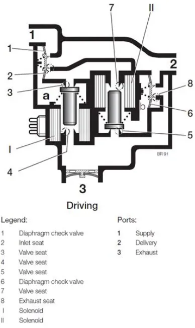
Fig 1 shows the pressure control valve which is an electro pneumatic control valve that contains solenoid used for controlling air pressure. The modulator valve is a solenoid-controlled air valve, consisting of two electrically operated solenoids and three diaphragm valves. The ECU controls the solenoids, which are extremely fast acting. They control pressure on the diaphragms, which then open or close passages to supply pressure to, or exhaust pressure from, the brake chamber.
Working of Pressure Control Valve
During normal braking, both solenoids in the ABS modulator valve are de-energized or inactive. The braking pressure applied at port 1 pressurizes the diaphragm (1) so that inlet seat (2) opens. Braking pressure gets into the chamber (b) via valve seat (7). The exhaust seat (8) remains closed and port 2 delivers the same pressure at port 1 to the service brake actuators. The ABS valve maintains this balanced (or pressure increase) position until a wheel starts to lock. (Fig. 2)
ISSN: 0975-833X
International Journal of Current Research Vol. 9, Issue, 06, pp.52531-52541, June, 2017
INTERNATIONAL JOURNAL OF CURRENT RESEARCH
Article History:
Received 23rdMarch, 2017
Received in revised form 07thApril, 2017
Accepted 15thMay, 2017
Published online 30thJune, 2017
Citation: Vinit Shete, Ketan Parashar, Shashank Borde and Nandgaonkar, M. R. 2017.“CFD analysis of pressure control valve used in abs using fluid
structure interaction technique”,International Journal of Current Research, 9, (06), 52531-52541.
Key words:
Fluid Structure Interaction, FSI, ABS,
Valve,
Diaphragm, Deformation, Mesh.
RESEARCH ARTICLE
CFD ANALYSIS OF PRESSURE CONTROL VALVE USED IN ABS USING FLUID STRUCTURE
INTERACTION TECHNIQUE
*Vinit Shete, Ketan Parashar, Shashank Borde and Nandgaonkar, M. R.
1
Dept of Mechanical Engineering, College of Engineering, Pune, India
2Project leader, Knorr-bremse Technical Centre India, Pune, India
3Technical Specialist, Knorr-bremse Technical Centre India, Pune, India
4
Associate Professor, Dept of Mechanical Engineering, College of Engineering, Pune, India
ARTICLE INFO ABSTRACT
The pressure control valve is an important part of the antilock braking system (ABS). The functioning of ABS depends upon the response of this valve and mainly upon the diaphragms used in this valve. There are three diaphragms in the valve which deform due to the air pressure at different stages of the valve operation. Thus, it is required to simulate the exact operating conditions of the valve using modern simulation techniques and try to optimize the performance of the valve. Fluid Structure Interaction (FSI), one of the modern simulation techniques is used in the ANSYS software to replicate the exact operating conditions of the valve and find the exact deformation of the diaphragms. The type of simulation currently used for the valve does not take into account the interaction between the air and the diaphragm. In this paper, different turbulent models are used for the steady state simulation and mesh independent study is presented. From the results, Shear State Transport model and a fine mesh with 5.7 million elements have been selected and steady state analysis is carried out. The one way FSI method which is a steady state technique has been used to find the deformation of the diaphragm. The difference between the simulation of the valve using FSI and without using FSI is presented. The deformation of the diaphragm is 3.42 mm. The change in deformation with the change in mass flow rate is also presented.
Copyright©2017, Vinit Shete et al. This is an open access article distributed under the Creative Commons Attribution License, which permits unrestricted use,
distribution, and reproduction in any medium, provided the original work is properly cited.
INTRODUCTION
An anti-lock braking system (ABS) is an automobile safety system that allows the wheels on a motor vehicle to maintain tractive contact with the road surface according to driver inputs while braking, preventing the wheels from locking up (ceasing rotation) and avoiding uncontrolled skidding. It is an automated system that uses the principles of threshold braking and cadence braking which were practiced by skillful drivers with previous generation braking systems [Chinmaya, 2007]. It does this at a much faster rate and with better control than a driver could manage. ABS generally offers improved vehicle control and decreases stopping distances on dry and slippery surfaces; however, on loose gravel or snow-covered surfaces, ABS can significantly increase braking distance, although still improving vehicle control. There are four main components of ABS: wheel speed sensors, valves, a pump, and a controller.
*Corresponding author: Vinit Shete
Dept of Mechanical Engineering, College of Engineering, Pune, India.
Fig 1 shows the pressure control valve which is an electro pneumatic control valve that contains solenoid used for controlling air pressure. The modulator valve is a solenoid-controlled air valve, consisting of two electrically operated solenoids and three diaphragm valves. The ECU controls the solenoids, which are extremely fast acting. They control pressure on the diaphragms, which then open or close passages to supply pressure to, or exhaust pressure from, the brake chamber.
Working of Pressure Control Valve
During normal braking, both solenoids in the ABS modulator valve are de-energized or inactive. The braking pressure applied at port 1 pressurizes the diaphragm (1) so that inlet seat (2) opens. Braking pressure gets into the chamber (b) via valve seat (7). The exhaust seat (8) remains closed and port 2 delivers the same pressure at port 1 to the service brake actuators. The ABS valve maintains this balanced (or pressure increase) position until a wheel starts to lock. (Fig. 2)
ISSN: 0975-833X
International Journal of Current Research Vol. 9, Issue, 06, pp.52531-52541, June, 2017
INTERNATIONAL JOURNAL OF CURRENT RESEARCH
Article History:
Received 23rdMarch, 2017
Received in revised form 07thApril, 2017
Accepted 15thMay, 2017
Published online 30thJune, 2017
Citation: Vinit Shete, Ketan Parashar, Shashank Borde and Nandgaonkar, M. R. 2017.“CFD analysis of pressure control valve used in abs using fluid
structure interaction technique”,International Journal of Current Research, 9, (06), 52531-52541.
Key words:
Fluid Structure Interaction, FSI, ABS,
Valve,
Fig. 1. Pressure Control Valve
Fig. 2. Operational framework of pressure control valve
By energizing the solenoid (I) the valve seat (4) is closed and valve seat (3) is opened. This supplies air to chamber (a) and inlet seat (2) is closed by the diaphragm check valve (1).The exhaust seat (8) also remains closed due to the pressure in chamber (b). The pressure at port 2 is held (neither increased nor reduced)By energizing the solenoid (I) the valve seat (4) is closed and the valve seat (3) is opened. Compressed air flows into the chamber (a) so that the diaphragm check valve (1) closes the inlet seat (2). The solenoid (II) is also energized and it closes valve seat (7) and opens valve seat (5).The pressure in chamber (b) exhausts through the now open valve seat (5). The diaphragm check valve (6) opens the exhaust seat (8) due to the brake chamber pressure (port 2) and this pressure is reduced via the exhaust port 3.The solenoids (I, II) are de-energized. This reduces the pressure in chamber (a) via the valve seat (4) and inlet seat (2) opens.
Air is supplied to chamber (b) via the valve seat (7) which closes exhaust seat (8). The braking pressure at port 2 increases again.
METHODOLOGY
As explained in the introduction, the optimal performance of the pressure control valve depends upon the reaction time of the diaphragms. The extent of opening of the diaphragm depends upon the mass flow rate through the valve. Numerical tool is used for investigation and analysis of the behavior of the diaphragms by applying essential boundary conditions and fluid properties. The numerical analysis is performed under steady environment using the fluid structure interaction technique to find the exact deformation of the diaphragm under working conditions.
Literature review
Basic Governing Equations
The various theoretical equations that govern the numerical analysis are discussed as follows:
Continuity Equation
A continuity equation describes the transport of a conserved quantity. Continuity equation also defined as conservation of mass. The law of conservation of mass state that mass can neither be created nor be destroyed. Three dimensional, incompressible, unsteady, continuity equations are as follows:
(1)
Momentum Equation
The Navier-Stokes equations are the basic governing equation for viscous, heat conducting fluid. It is a vector equation
obtained by applying newton’s law of motion to a fluid
element and is also called the momentum equation. Navier-stoke equation considers the viscosity of fluid because in most cases we cannot neglect the viscous effect.
x-component of momentum equation is,
y-component of momentum equation is,
z-component of momentum equation is,
Where,
p - static pressure,
u, v, w - velocity components in x, y and z direction. - dynamic viscosity
[image:2.595.66.260.259.585.2]- momentum source
Energy Equation
The energy of a fluid is defined as the sum of internal (thermal) energy i, kinetic energy and gravitational potential energy. The conservation of the energy of the fluid particles is ensured by equating the rate of change of energy of the fluid to the sum of the net rate work done on the fluid particle, the net rate of heat rate addition to the fluid and the rate of increase of energy due to source.
The energy equation is,
Turbulence Modelling
A turbulence model is a computational procedure to close the system of mean flow equations so that a relatively wide variety of flow problems can be calculated. The shear state transport k-ω turbulence model is a predominant two-equationeddy-viscosity model widely used. The use of a k-ω formulation in
the inner parts of the boundary layer makes the model directly usable all the way down to the wall through the viscous sub-layer hence the SST k-ω model can be used as a Low-Re turbulence model without any extra damping functions. The SST formulation also switches to k-ε behavior in the free -stream and thereby avoids the common k-ω problem that the
model is too sensitive to the inlet free-stream turbulence properties.
For turbulent kinetic energy k,
For specific dissipation rateω,
Computational setup
Computational Domain
In the PCV, there are 3 ports; inlet, outlet and exhaust. In the third stage of operation of PCV i.e. the pressure release stage wherein the air gets exhausted to the atmosphere, the air travels from the outlet port to the exhaust port. Thus, only the path through which air travels while moving from outlet port to the exhaust port has been chosen for the analysis and has been extracted from the original geometry. The diaphragm which is present near the exhaust port of PCV is chosen for the present work as the operating conditions of the three diaphragms are the same. Hence, the same simulation settings can be applied for the other two diaphragms
The fluid volume extracted from the original geometry is shown in fig. 3.
Meshing
[image:3.595.345.510.54.444.2]After extracting the fluid volume, the model is meshed in Ansys meshing as shown in Fig. 4 and the effect of boundary layer, is applied using inflation.
Fig. 3. Fluid Domain of the PCV
[image:3.595.37.233.463.535.2]Fig. 4. Mesh model for fluid flow (CFX)
Fig. 5. Geometry for static structural module
[image:3.595.364.506.564.664.2]The first layer height option is selected in inflation and all the faces except inlet and outlet are selected for inflation. The growth rate is kept to 1.2 and the numbers of layers are set to 6.
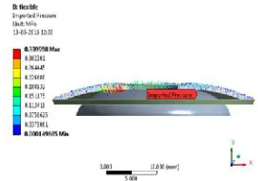
Fig. 6. Imported pressure on diaphragm
Boundary Conditions
The boundary conditions for the PCV are applied with opening pressure at inlet which simulates the reservoir pressure and static pressure at outlet which simulates the atmospheric pressure.
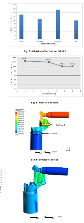
Fig. 7. Selection of turbulence Model
Fig. 8. Selection of mesh
Fig. 9. Pressure contour
Fig. 10. Y-plus
Diaphragm 1
[image:4.595.169.424.48.380.2]In the present work, air as an ideal gas is used as the fluid because the pressure at inlet is about 11 bar and air behaves as an ideal gas at such a high pressure. Also, using ideal gases (e.g. Air Ideal Gas) instead of constant density gases (e.g. Air at 25 C) gives a more stable solution. For a given interface displacement, an incompressible fluid responds with a higher pressure change than a compressible one. Even if the constant density assumption is valid for the converged solution, it can lead to divergence while iterating. In case of closed volumes, a compressible fluid must be used to conservemass.
Fluid Structure Interaction Setup
For the 1 way FSI method, the steady state results obtained are transferred to static structural module to obtain the interaction between diaphragm and air. From the geometry imported in structural setup, only the diaphragm and its supporting plate are kept as shown in fig. 5 and rest all the parts are suppressed as the main interaction of air would be with the diaphragm only.After meshing, the model is constrained with supports. The diaphragm is given fixed support on its internal face so that it will not move due to fluid pressure and will only deform. The plate is given remote displacement with all its degrees of freedom set to zero so that it remains constrained to its position. The pressure from the fluid flow gets imported into structural setup and acts on the diaphragm as the coordinate system of the geometry in CFX setup and the structural setup is same. Hence, the pressure developed during the fluid flow acts as imported load on diaphragm as shown in Fig. 6.
Selection of turbulence model
In the present work, different turbulence models like shear state transport, k-epsilon, k-omega and RNG k-epsilon are studied. Mass flow rate monitor is used for selection of the model. The iteration at which the mass flow at inlet and outlet becomes equal is compared for different models and the model for which the iterations are the least is chosen.From the fig 7, it is evident that Shear State Transport model is the best of all the other models as the mass flow rate for SST model becomes equal at inlet and outlet in 100 iterations which are the least. This is because SST uses of a k-ω formulation in the inner
parts of the boundary layer making the model directly usable all the way down to the wall through the viscous sub-layer hence the SST k-ω model can be used as a Low-Re turbulence model without any extra damping functions. The SST formulation also switches to k-ε behaviour in the free-stream and thereby avoids the common k-ω problem that the model is
too sensitive to receive the inlet free stream turbulence properties. Computational timing does not vary much in the above turbulence models.
Mesh Independent Study
In CFD, it generally happens that a solution gets converged with residuals well within the limit but if we further refine the mesh, the results obtained will be different. Hence, it is required to carry out a mesh independent study in which a mesh is refined up to a stage where there is not much variation in results and it can be said that the solution is independent of mesh size. The table I shows the different sizes of mesh that are used
The four different mesh sizes are simulated using the shear state transport model and the mass flow rate monitor is used for the selection in the same way as the turbulence model is selected. From the fig 8, it is observed that the iterations at which mass flow rate became constant is almost same for the fine and the finer mesh. Hence, it can be concluded that the fine mesh size is sufficient and no further refinement is required.
Pressure and Velocity Distribution
The pressure given at the inlet of the valve is 11 bar while at the outlet there is atmospheric pressure. The fig 9 shows the pressure distribution on the entire valve body. The reference pressure of 1 bar is set in the solver parameters. Hence, the inlet pressure is 10 bar and the outlet pressure is 0 bar.It can be observed that in the region of diaphragm 1, there is sudden change in direction of flow by about 1800. Hence, the air exerts pressure of about 7.9 bar in the region of diaphragm but due to change in direction there is a reduction of 42% in pressure and it drops to 4.6 bar once the air flows past the diaphragm. Again as the flow reaches the diaphragm 2, it exerts a pressure of 1.2 bar on the diaphragm 2 because the flow changes direction by 1800 once again. Thus, there is decrease of 72% in pressure from diaphragm 1 to diaphragm 2. The mass flow rate value at inlet obtained from the CFD-post is 0.112 kg/m3while that at the outlet is -0.112 kg/m3. This shows that entire quantity of air that has entered the domain has been obtained at the outlet. This suggests that the solution has converged well.
Y-plus
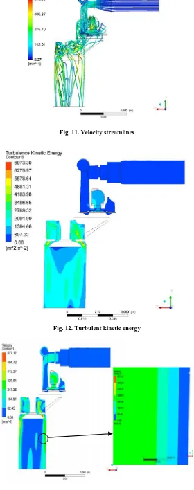
The y-plus values should be within the permissible value of 300. From the y-plus contour shown in fig 10, it can be observed that the y-plus values are well within the range. The maximum value of y-plus for the domain is 251.3 which is within the permissible limit. This shows that the velocity and pressure contours of the model have been resolved well. The higher values of y-plus around 200 to 250 are observed where there are sharp curves in the geometry. Most of the sharp curves have been smoothened in the design modeller before meshing but there are certain points where no changes can be made which are very few in the domain. Rest of the geometry have low values of y-plus as can be observed in the fig 10.The fig 11 shows the velocity streamlines which depict the flow pattern of the air in the domain.
Fig. 11. Velocity streamlines
Fig. 12. Turbulent kinetic energy
increases and becomes equal to free stream velocity at the outlet which is equal to 181 m/s. This distance from the wall at which the velocity becomes equal to the free stream velocity is called as the boundary layer thickness. In this case, the boundary layer thickness is 2 mm.The fig 14 shows the velocity variation of a turbulent flow with respect to the distance from the wall at the inlet. It can be seen from the graph that the velocity varies exponentially with the distance from the wall. It depicts the actual boundary layer phenomenon as explained earlier. The boundary layer thickness of 2 mm can be clearly observed from the fig 14. At a value of 0.033 m, the velocity is zero which is the wall surface. As the distance from the wall increases, the velocity increases and at a distance of 0.035 m, the velocity increases suddenly and becomes equal to the free stream velocity of 25.6 m/s at the inlet.
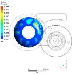
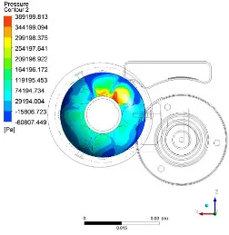
[image:7.595.178.423.234.482.2]The force acting on the diaphragm is shown in the fig 15. It can be observed from the fig 15 that the maximum force acts in the region where the air comes from the opening present just above the diaphragm and hits the diaphragm which is a small area. The maximum force is 0.4 N. The force acting in other regions is around 0.04 N to 0.16 N which is very less. The pressure acting on the diaphragm is shown in the fig 16. It can be observed that the maximum pressure acting on the diaphragm is 3.8 bar which is concentrated over a small area and pressure acting in other areas is relatively lesser between 1 to 2 bar. Hence, the deformation of the diaphragm is higher in the region where the pressure acting is the maximum. This deformation can be obtained through the FSI technique. The pressure obtained through the fluid flow in CFX is directly
Fig. 14. Velocity variation with distance from wall for turbulent flow
[image:7.595.172.422.512.767.2]Fig. 16. Pressure acting on the diaphragm
Fig. 17. Deformation of diaphragm with pressure inlet
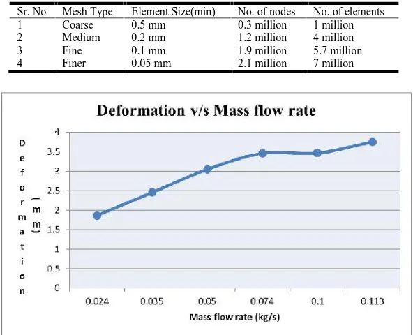
[image:8.595.141.466.601.786.2]Table 1. Mesh Independent Study
Sr. No Mesh Type Element Size(min) No. of nodes No. of elements
1 Coarse 0.5 mm 0.3 million 1 million
2 Medium 0.2 mm 1.2 million 4 million
3 Fine 0.1 mm 1.9 million 5.7 million
[image:9.595.154.424.351.538.2]4 Finer 0.05 mm 2.1 million 7 million
[image:9.595.166.408.569.756.2]Fig. 19.Variation of deformation of diaphragm with mass flow rate
Fig. 20. Uniform Pressure applied on diaphragm
applied to the diaphragm in the static structural module and the actual deformation obtained is shown in the fig 17.
Deformation of diaphragm using FSI
The flow that was developed in CFX is transferred to the structural setup to obtain the deformation of diaphragm as shown in Fig 17. It can be observed that the deformation is not uniform because the geometry of the valve is such that due to high velocity, major part of the air flows through the outer side of the diaphragm and there is no substantial deformation on the inner side. The maximum deformation of diaphragm is 3.4234 mm. The Fig 17 show that more pressure acts on one side of the diaphragm due to which it deforms non-uniformly. Thus, if the geometry is modified in such a way that the air comes in contact with the diaphragm more uniformly, it will apply uniform pressure on it and the deformation will be uniform. This may improve the life of valve. The inlet condition for the pressure control valve depends upon the application of brake by the driver. The maximum pressure supplied by the compressor to the PCV when brake pedal is pressed fully is 11 bar and hence, the maximum mass flow rate will never go beyond the value 0.113 kg/s. But, if the brake pedal is pressed partially, the mass flow rate will be less than 0.113 kg/s and hence, it is important to understand the trend of the deformation of diaphragm for different values of mass flow rate.
The fig 18 shows the variation of pressure exerted on diaphragm with increase in the mass flow rate with a maximum value of 0.113 kg/s. The figure shows the variation of pressure acting on the diaphragm for six different values of the mass flow rate varying from 0.024 kg/s to 0.113 kg/s. It can be observed that pressure increases almost linearly with the increase in mass flow rate. The fig 19 gives the variation of deformation of diaphragm with the increase in mass flow rate with a maximum value of 0.113 kg/s.It can be observed from the fig 19 that the for the least mass flow rate of 0.024 kg/s, the deformation is 1.8676 mm. It increases linearly up to a mass flow rate of 0.074 kg/s at which the deformation is 3.4589 mm. After this point, there is only 8% increase in deformation for 53% increase in mass flow rate. Thus, overall from fig 19 it can be said that deformation increases almost by 100% for an increase in mass flow rate from 0.024 kg/s to 0.113 kg/s which is maximum.
Advantage of FSI
The advantage of FSI is that the actual deformation of the diaphragm can be obtained only through FSI method. The fig 20 shows the uniform pressure of 0.12 MPa applied on the diaphragm. The uniform deformation of the diaphragm is shown in fig 21.
It can be observed from the fig 21 that under a uniform pressure of 0.12 MPa, a uniform deformation of 6.7942 MPa can be obtained.
Fig 20 and fig 21 clearly show that if only static structural analysis of the diaphragm is done, uniform pressure can be applied on it and the deformation obtained is also uniform which is not actual. With the FSI technique, it is possible to apply the non-uniform pressure that acts on the diaphragm in real conditions and the actual deformation shown in fig 17 can
be obtained. The fig 21 shows that under a uniform pressure, the diaphragm deforms up to 6.79 mm but the actual deformation found using FSI is only 3.4234 mm as shown in fig 17 which is 50% less.
DISCUSSION
The following points can be concluded from the above analysis:
For faster convergence, four different turbulent models are studied and compared using the mass flow monitor and mesh independent study has been carried out.
The recommended mesh size element is fine mesh having 5.7 million elements with body sizing of 2 mm, face sizing of 1.5 mm and inflation with first layer thickness of 0.06 mm and growth rate of 1.2 for 6 layers.
The Shear State Transport model is selected as the turbulence model as it converged faster than the other models and also, it is very practical in many industrial complex problems and also gives better and faster results.
The pressure contour shows that there is a reduction of 42% in pressure in the region of diaphragm 1 while there is decrease of 72% in pressure from diaphragm 1 to diaphragm 2.
The mass flow rate value at inlet obtained from the CFD-post is 0.112 kg/m3while that at the outlet, it is -0.112 kg/m3which is equal to the theoretical mass flow rate. This suggests that the solution has converged well.
The velocity streamlines show that the maximum velocity of 543 m/s occurs at the point just above the diaphragm it applies a force of 0.4 N on the diaphragm to open it.
There is a 233% increase in turbulent kinetic energy at the point where the flow comes in contact with the diaphragm.
The maximum deformation of the diaphragm is 3.4234 mm. This deformation is not uniform because the geometry of the valve is such that due to high velocity, major part of the air flows through the outer side of the diaphragm and there is not much deformation on the inner side.
For an increase in mass flow rate from 0.024 kg/s to 0.113 kg/s which is the maximum, there is a 100% increase in the deformation of diaphragm.
With the FSI technique, it is possible to apply the non-uniform pressure that acts on the diaphragm in real conditions and the actual deformation can be obtained. Under a uniform pressure, the diaphragm deforms up to 6.79 mm but the actual deformation found using FSI is only 3.4234 mm which is 50% less.
REFERENCES
Ayman A. Aly, El-Shafei Zeidan, Ahmed Hamed, Farhan
Salem, “An Antilock-Braking Systems (ABS) Control: A
Technical Review,” Intelligent Control and Automation, 2011, 2, 186-195 doi:10.4236/ica.2011.23023 Published Online August 2011.
Chinmaya B. Patil and Raul G. Longoria, “Modular design and testing for anti-lock brake actuation and control using a
Emil Boqvist: Investigation of a Swing Check Valve using CFD; ISRN: LIU-IEI- TEK-A—14/02013
Ismail B. Celik, “Introductory Turbulence Modelling,” West
Virginia University, Mechanical & Aerospace Engineering Dept, December 1999
Rugonyi, S., K. J. Bathe1, “On Finite Element Analysis of Fluid Flows Fully Coupled with Structural Interactions,”
CMES, vol.2, no.2, pp.195-212, 2001.
Versteeg H K, Malalasekera W, “Introduction To Computational Fluid Dynamics The Finite Volume Method,”(Longman, 1995) (T) (267S)