Statistical computation with kernels

(1)

warwick.ac.uk/lib-publications

A Thesis Submitted for the Degree of PhD at the University of Warwick

Permanent WRAP URL:

http://wrap.warwick.ac.uk/130103

Copyright and reuse:

This thesis is made available online and is protected by original copyright.

Please scroll down to view the document itself.

Please refer to the repository record for this item for information to help you to cite it.

Our policy information is available from the repository home page.

(2)

Statistical Computation with Kernels

by

Fran¸

cois-Xavier Briol

Thesis

Submitted to the University of Warwick

for the degree of

Doctor of Philosophy

University of Warwick,

Department of Statistics

(3)

List of Figures

1.1 Monte Carlo, importance sampling, Markov chain Monte Carlo and quasi-Monte Carlo (Halton sequence) point sets. . . 7

1.2 Closed Newton-Coates, open Newton Coates and Gauss-Legendre

point sets. . . 12

2.1 Sketch of a Gaussian process prior and posterior. . . 38

2.2 Importance of model selection for Gaussian processes. . . 40 2.3 Ill-conditioning of the Gram matrix in Gaussian process regression. . 43

3.1 Sketch of Bayesian quadrature. . . 52

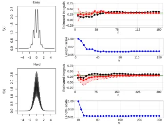
3.2 Test functions for evaluation of the uncertainty quantification pro-vided by Bayesian Monte Carlo and Bayesian quasi-Monte Carlo. . . 69

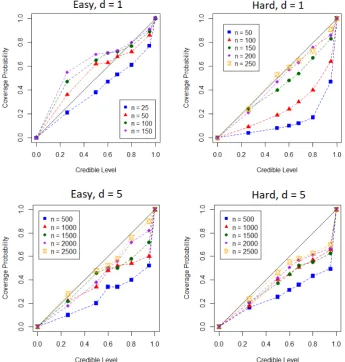
3.3 Coverage of Bayesian Monte Carlo (with marginalisation) on the test

functions . . . 71 3.4 Coverage of Bayesian Monte Carlo (without marginalisation) on the

test functions. . . 72

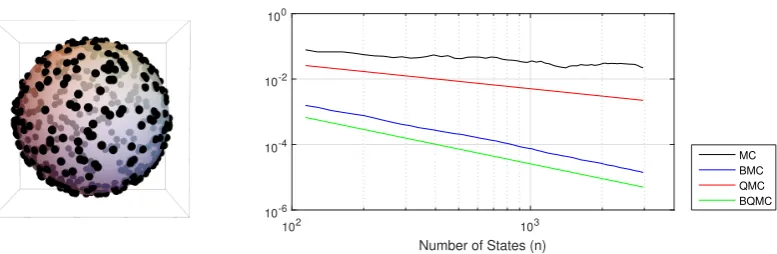
3.5 Convergence rates for Bayesian Monte Carlo and Bayesian quasi-Monte Carlo. . . 74

3.6 Posterior integrals obtained through Bayesian quadrature for

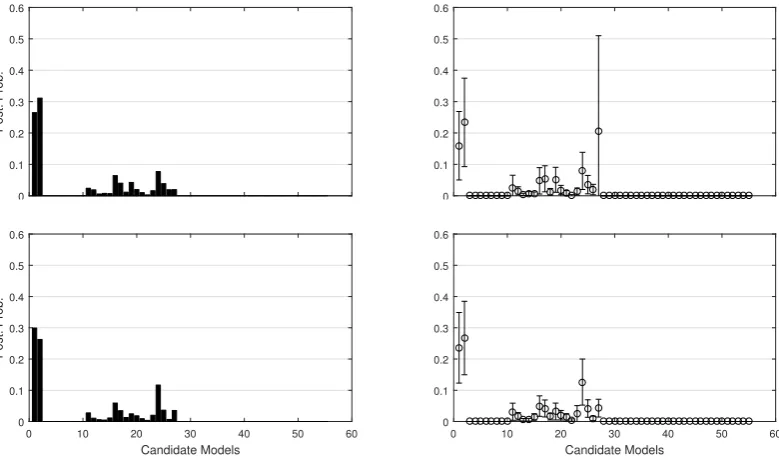
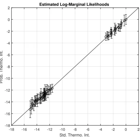
ther-modynamic integration in model selection . . . 79 3.7 Calibration of Bayesian quadrature for thermodynamic integration in

model selection . . . 80 3.8 The Teal South oil field. . . 81

3.9 Bayesian Markov chain Monte Carlo estimates of posterior means on

the parameter of the Teal South oil field model (centered around the exact values) . . . 82

3.10 Bayesian quasi-Monte Carlo for semi-parametric random effects

(7)

3.12 Bayesian quadrature estimates of the red, green and blue colour

in-tensities for the California lake environment. . . 88 3.13 Worst-case error of Bayesian Monte Carlo and Bayesian quasi-Monte

Carlo for global illumination integrals. . . 89

4.1 Test functions and Gaussian process interpolants in multi-fidelity modelling. . . 101

4.2 Uni-output and output Bayesian quadrature estimates for

multi-fidelity modelling. . . 102 4.3 Uni-output and multi-output Bayesian quadrature estimates in the

global illumination problem. . . 103

4.4 Frank-Wolfe algorithm on test functions. . . 110 4.5 Quantifying numerical error in a model selection problem using

Frank-Wolfe Bayesian Quadrature. . . 111

4.6 Comparison of experimental design-based quadrature rules on the proteomics application. . . 113

4.7 Influence of the importance distribution in Bayesian importance sam-pling. . . 115

4.8 Sensitivity of Bayesian importance sampling to the choice of both the

covariance function and importance distribution. . . 116 4.9 Lack of robustness of experimental-design based quadrature rules. . 118

4.10 Implementation of the stopping criterion for sequential Monte Carlo

Bayesian quadrature. . . 120 4.11 Performance of Sequential Monte Carlo Bayesian quadrature on the

running illustration. . . 123

4.12 Histograms for the optimal (inverse) temperature parameter on the illustrative example. . . 123

4.13 Sensitivity of sequential Monte Carlo Bayesian quadrature to the

choice of initial distribution and to the random number generator. . 125 4.14 Performance of sequential Monte Carlo Bayesian quadrature for

syn-thetic problems of increasing complexity. . . 125

4.15 Performance of Sequential Monte Carlo Bayesian quadrature on the running illustration in increasing dimensions. . . 126

4.16 Performance of sequential Monte Carlo Bayesian quadrature for an

inverse problem based on an ordinary differential equation. . . 127

(8)

5.2 Descent trajectories of gradient descent and natural gradient descent

algorithms on a one-dimensional Gaussian model for estimators based on the KL, SM and KSD divergences. . . 162

5.3 Performance of natural gradient descent algorithms on a 20-dimensional

Gaussian model for estimators based on the KL, SM and KSD diver-gences . . . 163

5.4 Maximum mean discrepancy estimator based on a Gaussian RBF

kernel for a Gaussian location model. . . 164 5.5 Maximum mean discrepancy estimator based on a Gaussian RBF

(9)

Acknowledgments

I am first and foremost grateful to my advisor, Mark Girolami, for giving me

op-portunities which are usually reserved to researchers in later stages of their careers.

He introduced me to exciting areas of research across the fields of statistics, applied

mathematics and machine learning, and to researchers doing interesting work in

these areas. Mark also gave me the opportunity to attend conferences which greatly

enriched my PhD experience and broadened my overview of statistics research.

Fi-nally, he has always been a great mentor, and regularly taken the time to make sure

my PhD was running smoothly.

Of course, most of my work would not have been possible without the

sup-port and guidance of Chris Oates, who I consider as a great mentor and unofficial

second advisor. Chris has been very patient in answering many of my mathematical

questions, and taught me how to structure my research in an effective way.

I would also like to express my gratitude to many of the faculty members,

students and visitors at the various institutions I have attended during my PhD,

including the University of Oxford, University of Warwick, Imperial College London

and The Alan Turing Institute. I am in particular grateful to all of the lecturers

and students in the first year of the Oxford-Warwick Statistics programme which I

have greatly enjoyed. I am also thankful to Michael Osborne and Dino Sejdinovic

who have initiated me into the world of machine learning, Andrew Duncan and

Alessandro Barp who have greatly widened my understanding of mathematics, and

Jon Cockayne, Louis Ellam and Thibaut Lienart who have been of great help in

an-swering many of my questions about statistics, machine learning and programming.

(10)

(SIAM), the American Statistical Association (ASA), the Statistical and Applied

Mathematical Sciences Institute (SAMSI) and the International Society for Bayesian

Analysis (ISBA) for several travel awards which funded some of my travels to

in-ternational conferences. I have also been fortunate to have the opportunity to visit

several universities across the world, including a week-long visit at the University

of Technology Sydney hosted by Chris Oates and Matt Wand, a month-long visit

at the California Institute of Technology hosted by Andrew Stuart and Houman

Owhadi, and a three week visit at the Isaac Newton Institute at the University of

Cambridge, where I was hosted by Catherine Powell. To all my hosts: thank you.

Finally, I would also like to thank Wilfrid Kendall and Arthur Gretton for

(11)

Declarations

This thesis is submitted to the University of Warwick in support of my application

for the degree of Doctor of Philosophy. It has been composed by myself and has

not been submitted in any previous application for any degree. The work presented

(including data generated and data analysis) was carried out by the author except

in the cases outlined below. Parts of this thesis have been published by the author:

1. F-X. Briol, C. J. Oates, M. Girolami, and M. A. Osborne. Frank-Wolfe

Bayesian quadrature: Probabilistic integration with theoretical guarantees.

InAdvances In Neural Information Processing Systems 28, pages 1162–1170,

2015a

. The article was mostly written by Chris Oates and myself, and we both contributed equally to the methodology and theory sections. The numerical

experiments were done by myself, with some code from a previous publication

contributed by Chris Oates. Mark Girolami and Michael Osborne provided

helpful suggestions to improve the manuscript. The paper was awarded a

“spotlight presentation” at NIPS 2015, which was only awarded to the top

4.5% of submitted papers.

2. F-X. Briol, C. J. Oates, M. Girolami, M. A. Osborne, and D. Sejdinovic.

Proba-bilistic integration: A role in statistical computation?To appear in “Statistical

Science” with discussion and rejoinder, arXiv:1512.00933, 2015b

. The article was mostly written by Chris Oates and myself, and we both

contributed equally to the methodology and theory sections. The numerical

(12)

also contributed by Chris Oates, Shiwei Lan and Ricardo Marques.

The paper was awarded a “Best Student Paper” award in 2016 by the

sec-tion on Bayesian Statistical Science of the American Statistical Associasec-tion,

and was reviewed in a series of blog posts by eminent statisticians

includ-ing Andrew Gelman: http://andrewgelman.com/2015/12/07/28279/and

Christian Robert https://xianblog.wordpress.com/2015/12/17/. It has

been accepted to “Statistical Science”, and will appear with discussions from

leading statisticians (including Michael L. Stein, Ying Hung, Art Owen, Fred

Hickernell and R. Jagadeeswaran) and a rejoinder from the authors [Briol

et al., 2018].

3. F-X. Briol, J. Cockayne, and O. Teymur. Comments on “Bayesian solution

uncertainty quantification for differential equations” by Chkrebtii, Campbell,

Calderhead & Girolami. Bayesian Analysis, 11(4):1285–1293, 2016

.This paper is a contributed discussion of Chkrebtii et al. [2016], and is the outcome of a series of discussions between Jon Cockayne, Onur Teymur and

myself. The paper was mostly written by myself.

4. F-X. Briol, C. J. Oates, J. Cockayne, W. Y. Chen, and M. Girolami. On the

sampling problem for kernel quadrature. In Proceedings of the International

Conference on Machine Learning, pages 586–595, 2017

. This article is the result of collaborative work between Chris Oates and

myself. The numerical experiments were all performed by myself.

5. C. J. Oates, S. Niederer, A. Lee, F-X. Briol, and M. Girolami. Probabilistic

models for integration error in the assessment of functional cardiac models.

Advances in Neural Information Processing, 2017d

. This articles originates from discussions between Chris Oates and myself.

The articles and numerical experiments are Chris Oates’ work. Angela Lee

and Steven Niederer provided the application for the paper.

(13)

for statistical data science. In Statistical Data Science, pages 99–110. World

Scientific, 2018

. This article is a chapter in the book “Statistical Data Science” edited by

Niall Adams and Edward Cohen, and was written independently by myself.

7. A. Barp, F.-X. Briol, A. D. Kennedy, and M. Girolami. Geometry and

dy-namics for Markov chain Monte Carlo. Annual Reviews in Statistics and Its

Applications, 5, 2018

. The article was written by Alessandro Barp and myself, with suggestions and revisions by Anthony Kennedy and Mark Girolami.

8. C. J. Oates, J. Cockayne, F.-X. Briol, and M. Girolami. Convergence rates for

a class of estimators based on Stein’s identity. Bernoulli, 2018

.The article was mostly written by Chris Oates, who also developed most of the theory. Jon Cockayne contributed numerical simulations, and I helped

generalise the proofs.

9. X. Xi, F-X. Briol, and M. Girolami. Bayesian quadrature for multiple related

integrals. International Conference on Machine Learning, PMLR

80:5369-5378, 2018

. This article emanates from Xiaoyue Xi’s thesis project for the MSc in Statistics at Imperial College London, which was supervised by myself. The

project, methodology and theory were by all done by myself. Xiaoyue Xi

was in charge of numerical simulations. The article was accepted for a “long

talk” at ICML 2018, which was awarded to the top 8% of submitted papers.

10. W. Y. Chen, L. Mackey, J. Gorham, F-X. Briol, and C. J. Oates. Stein points.

InProceedings of the International Conference on Machine Learning, PMLR

80:843-852, 2018

. The idea was originally proposed by myself. Chris Oates wrote most of the paper, Wilson Chen performed the numerical experiments and Lester

(14)

11. F.-X. Briol, C. J. Oates, M. Girolami, M. A. Osborne, and D. Sejdinovic.

Rejoinder for “Probabilistic integration: a role in statistical computation?”.

Statistical Science (to appear), arXiv:1811.10275, 2018

.The article was written myself, with comments and feedback from all other

authors. It will appear as the rejoinder for Briol et al. [2015b], which will

appear with discussions at Statistical Science.

Chapter 5 is also part of ongoing work with Andrew Duncan, Alessandro Barp,

(15)

Abstract

Modern statistical inference has seen a tremendous increase in the size and complexity of models and datasets. As such, it has become reliant on advanced com-putational tools for implementation. A first canonical problem in this area is the numerical approximation of integrals of complex and expensive functions. Numerical integration is required for a variety of tasks, including prediction, model comparison and model choice. A second canonical problem is that of statistical inference for models with intractable likelihoods. These include models with intractable normal-isation constants, or models which are so complex that their likelihood cannot be evaluated, but from which data can be generated. Examples include large graphical models, as well as many models in imaging or spatial statistics.

This thesis proposes to tackle these two problems using tools from the kernel methods and Bayesian non-parametrics literature. First, we analyse a well-known algorithm for numerical integration called Bayesian quadrature, and provide consis-tency and contraction rates. The algorithm is then assessed on a variety of statistical inference problems, and extended in several directions in order to reduce its compu-tational requirements. We then demonstrate how the combination of reproducing kernels with Stein’s method can lead to computational tools which can be used with unnormalised densities, including numerical integration and approximation of probability measures. We conclude by studying two minimum distance estimators derived from kernel-based statistical divergences which can be used for unnormalised and generative models.

(16)

Abbreviations

BIS . . . .. . . .Bayesian importance sampling

BMC, BMCMC. . . .Bayesian Monte Carlo, Bayesian Markov chain Monte Carlo

BQ . . . .. . . .Bayesian quadrature

BQMC . . . .. . . .Bayesian quasi-Monte Carlo

FW, FWLS . . . .. . . .Frank-Wolfe, Frank-Wolfe with line search FWBQ . . . .. . . .Frank-Wolfe Bayesian quadrature

FWLSBQ . . . . .. . . .Frank-Wolfe with line search Bayesian quadrature GP . . . .. . . .Gaussian process

IID . . . .. . . .Identically and independently distributed IS . . . .. . . .Importance sampling

KL . . . .. . . .Kullback-Leibler

KSD . . . .. . . .Kernel Stein discrepancy

MC, MCMC . . .. . . .Monte Carlo, Markov chain Monte Carlo MMD . . . .. . . .Maximum mean discrepancy

QMC . . . .. . . .Quasi-Monte Carlo RBF . . . .. . . .Radial basis function

RKHS . . . .. . . .Reproducing kernel Hilbert space SM . . . .. . . .Score matching

SMC . . . .. . . .Sequential Monte Carlo

SMC-BQ . . . .. . . .Sequential Monte Carlo Bayesian quadrature

(17)

Chapter 1

Challenges for Statistical

Computation

“Computations are an issue in statistics whenever processing a dataset becomes a difficulty, a liability, or even an impossibility.”

Green et al. [2015]

As illustrated by Green et al. [2015], computation has always been an issue

for large-scale statistical inference. Recently, computational issues have been

exac-erbated by increases in computing resources and the availability of larger datasets, which has encouraged scientists to fit ever-more complex models. Keeping up with

these changes is a constant challenge for researchers in computational statistics. In

this thesis, we review some of the main problems in this area and contribute novel methodology to two of them: (i) the problem of numerical integration of complex

and expensive functions, and (ii) the problem of statistical inference for models with

intractable likelihoods.

1.1 Challenge I: Numerical Integration and Sampling

Let (X,F, µ) be a measure space1. A major issue preventing the application of many complex statistical methodologies is the need to compute the Lebesgue integral of

1

(18)

some integrable functionsf :X →_R:

Π[f] := Z

X

f(x)Π(dx), (1.1)

where Π is some probability measure on (X,F) assumed to admit some probability density functionπwith respect to some underlying reference measureµon the space

X. The space X is called the state space and is usually a subspace of Rd or some

manifold embedded in Rd for some d∈ N (where we adopt the convention that N

does not include 0).

From the point of view of statistical computation, the main issue arises when these integrals cannot be evaluated in closed form and have to be estimated

numeri-cally. Historically, classical quadrature rules such as Gaussian quadratures have been

used extensively [Naylor and Smith, 1982; Smith et al., 1985]. These are however only suitable for low-dimensional integrals with a smooth integrand. Nowadays,

it is common to use Monte Carlo (MC) methods [Meyn and Tweedie, 1993; Liu,

2001; Robert and Casella, 2004] to approximate the integral by taking an average of function values at samples from Π (either identically and independently distributed

(IID) or approximately IID).

In both of the cases above, we obtain an approximation of the form:

ˆ

Π[f] :=

n

X

i=1

wif(xi), (1.2)

called quadrature (or cubature) rule, based on point sets (also called samples)xi ∈ X

and weightswi ∈ Rfor i= 1, . . . , n. Under certain regularity conditions, this

esti-mator converges to the solution of the integral asn→ ∞. For finite but large sample sizes n, the estimator reasonably approximates the truth. However, these estima-tors will have (potentially very) large errors wheneverπ is highly multimodal, the state-spaceX is high-dimensional or the integrandf is computationally expensive to evaluate. Adapting numerical integration methods to each of these scenarios is one

of the main tasks in computational statistics. We now highlight several applications

of numerical integration in statistics.

1.1.1 Applications in Bayesian Statistics

In Bayesian statistics [Robert, 1994; Gelman et al., 2013], once a model and a prior have been specified, all that remains to be done is to repeatedly apply Bayes’ theorem

until we obtain a distribution on the variables of interest conditioned on every other

(19)

from some data space denotedDand byθ∈Θ the parameters of a statistical model. For simplicity, we assume that D and Θ are both Euclidean spaces. The simplest formulation of Bayesian inference (assuming the existence of all densities) is the

following equation2:

p(θ|X) = p0(θ)p(X|θ)

p(X) , (1.3)

wherep(X|θ) denotes the likelihood, or statistical model, and describes the plausi-bility of the parameter taking valueθwhenXis observed. Furthermore,p0(θ) is the

prior density on the unknown model parametersθandp(θ|X) denotes the posterior density (after having observed X) on these same parameters. The quantity in the

denominator,p(X) is called the model evidence or marginal likelihood, and can be expressed as

p(X) = Z

Θ

p(X|θ)p0(θ)dθ. (1.4)

The model evidence is an example of an integral that almost always needs to be computed, in this particular case in order to be able to evaluate our posterior on

parametersθ. This is not possible in all but special cases, in which case we call this Bayesian approach a conjugate analysis.

Integrals are also required when predicting new data valuesx0 ∈ D. This can

be done by computing the posterior predictive distribution

p(x0|X) = Z

Θ

p(x0|θ)p(θ|X)dθ, (1.5)

which allows us to propagate the uncertainty in our posterior through to predictions. Similar integrals are also required to do model selection with Bayes factors [Kass

and Raftery, 1995] or for Bayesian model averaging [Hoeting et al., 1999].

Clearly, Bayesian inference would be restricted to very simple models without numerical integration. This explains why Bayesian methods only became widely

popular across the sciences in the 1990s, at which point the statistics community

had been introduced to Markov Chain Monte Carlo (MCMC) methods [Robert and Casella, 2011].

2

(20)

1.1.2 Applications in Frequentist Statistics

Challenging integrals are also ubiquitous in frequentist statistics, and are often

required for maximum likelihood estimation. Suppose we have IID realisations

{xi}ni=1 ⊂ D from a probability measurePθ∗ from some parametric family of Borel

probability measures P_Θ(D) = {_P_θ :θ ∈Θ} defined onD. Once again assume D

and Θ are Euclidean spaces and denote by p(·|θ) the Lebesgue density of Pθ. We

are interested in finding the “true” parameter θ∗ ∈ Θ which generated these sam-ples, and the maximum likelihood approach proposes to do so by maximising the

expected log-likelihood under the data-generating process:

arg max

θ∈Θ

Z

D

logp(x|θ)p(x|θ∗)dx. (1.6)

In practice, the integral is usually approximated using a MC estimate with the

samples {xi}ni=1 that are readily available, and we get the following optimisation

problem:

arg max

θ∈Θ

1

n

X

i=1

logp(xi|θ). (1.7)

Numerical integration is therefore clearly fundamental here, and we may wish to

use more efficient methods to approximate the integral. Note that the approach is

of course only feasible if the likelihood can be evaluated in closed form. In the case of latent variable models, this does not necessarily hold. Indeed, assume we have a

set of unobserved variablesy(called nuisance parameters) in some spaceY. In this

case, we would usually have access to a conditional likelihoodp(x|y, θ) and therefore need to integrate out all possible values of the latent variabley to get a marginal

likelihood:

p(x|θ) = Z

Y

p(x|y, θ)p(y|θ)dy. (1.8)

which we can then use for maximum likelihood estimation. This will be infeasible

for most models and will once again require numerical integration; see Diggle et al.

(21)

1.1.3 Existing Methodology

The ubiquity of integration across statistics should now be clear to the reader. We

now move on to discuss how the problem of numerical integration can be tackled in

practice. In this section, we briefly review existing methodology, then discuss some of their shortcomings. Recall that we assume throughout this chapter that (X,F, µ) is a measure space and Π is a probability measure with density (with respect toµ) denotedπ.

Monte Carlo Integration and Importance Sampling

Monte Carlo methods are quadrature rules based on uniform weights. The simplest

of those methods, which is usually simply referred to as “Monte Carlo” [Robert and

Casella, 2004; Glasserman, 2004], consists of obtaining IID realisations {xMC_i }n i=1

from the measure Π and approximating Π[f] as:

ˆ

ΠMC[f] :=

1

n

X

i=1

f xMC_i

.

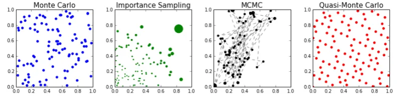
An illustration of such a point set is available in Figure 1.1 for the case where Π

is a uniform measure on the unit cube X = [0,1]2. MC estimators are popular in statistics owing to their wide applicability and their well-known properties. For

instance, under regularity conditions (omitted for brevity), the central limit theorem

gives that

√

nΠˆMC[f]−Π[f]

_D

−→ N(0,Varπ[f]), (1.9)

where −D→ denotes convergence in distribution. We use the notation N(m, c) to denote a normal distribution with meanm and covariancec, and Varπ[f] = Π[f2]−

Π[f]2 is the variance of f under Π. MC is well-suited to numerical integration problems since it provides a dimension-independent convergence rate ofOP(n−1/2)3.

A major limitation with MC is the need to sample IID realisations from Π,

which is only possible for a limited set of distributions. An alternative estimator with weighted point sets is called importance sampling (IS) and is of the form:

ˆ

ΠIS[f] := n

X

i=1

wIS_i f xIS_i

, (1.10)

3

We write that some functionf(x) isO(g(x)) if the statement “∃M, x0>0 such that|f(x)| ≤

(22)

where{xIS_i }n

i=1 are IID realisations from another probability measure Π0 called

im-portance measure. This imim-portance measure is defined on (X,F) and is specified a-priori by the user. Its density with respect to µ satisfies π0(x) > 0 whenever

π(x)f(x)6= 0, and the IS weights are given by:

wIS_i := π(xi)

nπ0₍_x i)

, (1.11)

for i = 1, . . . , n. The IS estimator in Equation 1.10 can be be seen as an MC estimator where the function f0(x) = f(x)π(x)/π0(x) is integrated with respect to the measure Π0. IS is most often used when IID sampling from Π is not feasible, or

because clever choices of importance distribution Π0 can lead to significant variance

reduction in the corresponding central limit theorem. However, IS tends to become inefficient in high dimensions when most samples will have near zero weight. This

is due to the fact that, in high dimensions, regions of high probability will tend to

be concentrated on small subsets of the sample spaceX (a phenomenon known as the curse of dimensionality; see [MacKay, 2003; Betancourt, 2017]).

An illustration of IS is given in Figure 1.1 (middle left), where IID

realisa-tions{xIS_i }n

i=1 are obtained from some importance measure Π0 which is a truncated

Gaussian centred at the origin. The size of the samples is plotted proportional to

their weight (as given by Equation 1.11). As observed, there are fewer realisations

in the top right corner, but these have larger weights. This compensates for the fact that Π0 has very low mass in that part of the domain. The choice of importance

distribution will be particularly efficient if the integrandf is such thatπ0(x)∝f(x). In this case, Π0 would be the optimal importance sampling distribution and the IS

estimator would have lower asymptotic variance than the MC estimator.

Markov Chain Monte Carlo Integration

Often we only know π, the density of Π, up to a multiplicative constant. That is, we are able to evaluate ˜π where π(x) = ˜π(x)/Z for some unknown Z ∈ R+.

This is for example the case in Bayesian statistics where the probability measure Π

is a posterior measure and the normalisation constant Z is the model evidence in Equation 1.4. In this case, neither MC or IS can be used, but MCMC methods [Meyn

and Tweedie, 1993; Robert and Casella, 2004] can be a useful alternative. The idea

behind MCMC is to generate correlated samples{xMCMC_i }n

i=1which, marginally, are

approximately IID realisations from the target measure Π by obtaining a realisation

(23)

[image:23.595.121.517.109.205.2]

Figure 1.1: Monte Carlo, importance sampling, Markov chain Monte Carlo and

quasi-Monte Carlo (Halton sequence) point sets. Plot of n = 100 points for each

algorithm for integration against a uniform distribution on [0,1]2.

then becomes:

ˆ

ΠMCMC[f] :=

1

n

X

i=1

f xMCMC_i . (1.12)

Recall that a Markov chain is a sequence of random variablesX0, X1, . . . such that

the distribution ofXiis only conditional onXi−1. A Markov chain may be specified

by an initial measureH0 (with densityh0) forX0 and a transition measureT, (with

densityt(·|x) :X →R+) from which we can sample. Xi is then a realisation from a

measure Hi with density given byhi(x0) =

R

Xt(x0|x)hi−1(x)dx. The measure Π is

called a stationary measure of the Markov chain if wheneverXiis a realisation from

Π, thenXi+1 is also a realisation from Π. This can be summarised succinctly with

the following condition: π(x0) = R

Xt(x0|x)π(x)dx. If the Markov chain is ergodic,

it will converge to its stationary measure independently of its initialisation.

The Metropolis-Hastings algorithm [Metropolis et al., 1953; Hastings, 1970] is the most widely used example of MCMC. It aims to construct a Markov chain

converging to the desired target measure Π by the means of a proposal kernel K :

X × X →[0,1], where for each x∈ X,K(·,x) is a probability measure with density

κ(·,x) :X →_R. The algorithm proceeds as follows. First, draw a realisationx0 ∈ X

fromH0. Then, at each iteration, given the current state xi∈ X:

1. Propose a new state ˜xby obtaining a realisation fromK(·,xi).

2. Accept the proposed state (i.e. set xi+1 = ˜x) with probability A(˜x|xi) :=

min n

1,_ππ_(xi)(˜x)κ_κ(xi_(˜_x_,,_xi)x)˜

o

, else keep the previous state (i.e. set xi+1 =xi).

(24)

a distributionT(·,x). When it exists, the density of T(·,x) is given by:

t(x0|x) := κ(x0,x)A(x0|x) + 1{x0_=x} 1−A(x0|x),

where 1{x0_=x}takes value 1 whenx0 =xand 0 otherwise. Note that the computation

ofA(x0|x) does not rely on the constant Z, due to a cancellation in the ratio. In principle, there are only mild requirements on the proposal kernel required to obtain an asymptotically correct algorithm. The choice of proposal kernel will

however have a high influence on the performance of the algorithm. Intuitively, the

aim is to choose a proposal kernel which will favour values with high probability of acceptance. Concurrently, we would also like the proposal kernel to be designed so

that chain explores the state space well in a small number of iterations, so that the realisations are as close to IID as possible.

A common choice is a symmetric distribution centred on the current state

of the chain, which gives the well-known random-walk Metropolis algorithm. This algorithm is illustrated in Figure 1.1 (middle right) where we have used a Gaussian

proposal centred at the current state and with variance 0.1. The black dots give the samples of the Markov chain and their size depends on the number of time they are repeated in the chain. On the other hand, the dotted lines indicate the path of

the chain. This example can highlight the difficulty of tuning Markov chains; the

chain is not very efficient at covering the whole space and this could most likely be resolved by increasing the variance of the proposal. It is also often possible to use

more efficient transition kernels.

A more advanced algorithm is the Metropolis-adjusted Langevin algorithm [Rossky et al., 1978; Scalettar et al., 1986; Roberts and Rosenthal, 1998], which

exploits gradients by approximating the path of a diffusion which is invariant to

the target distribution. Duane et al. [1987] also later proposed a method based on approximating Hamiltonian dynamics with potential energy given by the log

target density. This method was originally named Hybrid Monte Carlo, but is also

commonly known as Hamiltonian Monte Carlo [Neal, 2011; Betancourt, 2017; Barp et al., 2018]. Informally, these two methods have the advantage of using transition

kernels directing the Markov chain towards areas of high probability and are hence

preferable to the random-walk Metropolis algorithm above.

Another alternative to these algorithms is to restrict our proposal measure

to a parametric family of transition kernels. We then assume that a member of this

(25)

Haario et al., 2001; Andrieu and Thoms, 2008]. Adaptive MCMC algorithms can be

very efficient, but proving their correctness is difficult since the Markov property no longer holds since we are allowing the process to depend on more than the current

state.

Sequential Monte Carlo samplers

An approach which combines ideas from IS and MCMC are sequential Monte Carlo (SMC) methods. SMC (and other particle-based schemes) have had an enormous

in-fluence in signal processing, and more generally filtering and smoothing in a Bayesian

context [Doucet and Johansen, 2011; S¨arkk¨a, 2013]. More recently SMC algorithms have been proposed to sample from complex distributions, and these can be

partic-ularly efficient for multimodal target distributions.

SMC samplers [Chopin, 2002; Del Moral et al., 2006] start by defining a sequence of probability measures Π0,Π1, . . . ,ΠT where ΠT = Π is the measure we

would like to integrate against. The main idea behind SMC is to sequentially obtain

realisations from this sequence of measures by moving a set of particles. If Π0 is

simple to sample from, and moving particles across consecutive measures in this

sequence is also relatively easy, then SMC samplers can render the task of sampling

from Π manageable even when sampling from Π directly (e.g. using MCMC) would be difficult of even infeasible. The algorithm follows the following step. First,

we start by obtaining particles {xi}n_i₌₁ as IID realisations from Π0, then at each

iteration of the algorithm:

1. Update the weights using the formula for IS weights in Equation 1.11 with importance distribution Πt−1 and target Πt.

2. If some resampling criterion (described below) is satisfied, do a resampling

step. This means sampling (with replacement) from our current set of particles

according to their respective weights and setting the weights of the resampled particle to 1/n.

3. Update the particles using MCMC step(s) with invariant measure Πt.

Once iteration T is attained, a last resampling step is used to obtain a final set of equally-weighted particles which we will denote{xSMC_i }n

i=1. When this procedure is

completed, we end up with an estimator:

ˆ

ΠSMC[f] :=

1

n

X

i=1

(26)

The resampling strategy can be useful to avoid the degeneracy of particle weights

which is common with IS methods (i.e. most particles end up having near zero weight). The most common resampling approach is the multinomial sampling

de-scribed above, but alternatives can be more efficient [Douc et al., 2005].

Note that to avoid resampling at every step, it is common to use a criterion based on the variability of the current samples such as the effective sample size.

Another example, called conditional effective sample size, was proposed by Zhou

et al. [2016]. Given a set of weighted particles{xi, wi}ni=1 at iteration j, it can be

computed as:

CESS = n( Pn

i=1wizi)2

Pn

i=1wizi2

,

wherezi= (π(xi)/π0(xi))(tj−tj−1) fori= 1, . . . , nand π0 is the density of Π0.

Quasi-Monte Carlo Integration

All of the methods we have seen so far focus on approximating the target

mea-sure Π. When Π is simple, it is common to exploit properties of the integrands

instead. Quasi-Monte Carlo (QMC) methods [Dick and Pillichshammer, 2010; Dick et al., 2013] are estimators based on point sets with grid-like structures and

uni-form weights, usually defined on some domain X which is the unit cube and for

integration against a measure Π which is the uniform measure on this cube:

ˆ

ΠQMC[f] :=

1

n

X

i=1

fxQMC_i .

The point set{xQMC_i }n

i=1 is chosen to minimise some notion of discrepancy between

an empirical measure and the measure Π. For this reason, they are often referred

to as “space-filling designs”, and different notions of discrepancy lead to different QMC rules. These designs are either nested (i.e. the point set with n+ 1 points can be obtained by adding one point to the point set of size n) in which case they are called “open”, or non-nested (the point set of sizen+ 1 needs to be recomputed from scratch) in which case they are called “closed”.

An example of an open QMC point set is the Halton sequence, which is given

in the cased= 2 in red in Figure 1.1 (right). It can be observed that the sequence fills the space in a much more uniform way than the plot of MC points (in blue).

(27)

de-creases at the asymptotic rateO(n−1+) wheredenotes log terms. Specific methods have also been used to obtain fast convergence rates of O(n−αd+) in the classical

Sobolev spaces4 _Wα

2(X), where α denotes the number of weak derivatives of

func-tions in the space.

It is also well-known [Sloan and Wo´zniakowski, 1998] that QMC can perform particularly well in high dimensions; for example, a dimension-independent

con-vergence rate of O(n−α+) can be proved for Sobolev spaces of mixed dominating smoothness (usually denotedSα

2(X)).

Another direction of research has been randomised quasi-Monte Carlo which

proposes to randomise QMC point sets in a way which preserves their space-filling

properties. A particular example is the scrambling method of Owen [1997], which can also be shown to converge fast for smooth functions (in mean-squared error).

Although QMC methods can be used to obtain fast convergence rates, they

tend to be impractical for many applications due to their restriction to the cube and the uniform measure. Several ways of avoiding this issue have been proposed

in the literature, mostly focusing on transforming alternative problems to fit in this

setup, but these tend to be impractical.

Classical Deterministic Quadrature Rules

As already pointed out, another alternative which has historically been popular but

is now rarely used in modern statistical inference problems are classical deterministic

quadrature rules [Davis and Rabinowitz, 2007]. These rules are usually designed to integrate functions on some interval (a, b)⊂_R, and the weights and points are often chosen so as to integrate any polynomial up to a certain degree exactly.

The simplest examples include the midpoint rule, consisting of one point

x1 = (b−a)/2 and weightw1 =|b−a|, and the trapezoidal rule, consisting of the

two pointsx1=a, x2 =band weights w1 =w2 =|b−a|/2. The two rules integrate

exactly all polynomials of degree 0 and 1 respectively, and are part of the family of Newton-Cotes rules which are based on equally-separated points. These rules can be

either open5, in which case they integrate polynomials passing through all including the boundary exactly, or closed, in which case they do not evaluate integrands on

the boundary. See Figure 1.2 for an illustration.

Another class of quadrature rule, which can integrate polynomials of order up ton−1 withnpoints are the Gaussian quadrature rules [Golub and Welsch, 1969]. Different examples of Gaussian quadrature rules exist, depending on the measure

4

See Appendix A.1 for definitions and some additional background on functional analysis.

(28)

[image:28.595.176.465.110.203.2]

Figure 1.2: Closed Newton-Coates, open Newton Coates and Gauss-Legendre point

sets. Plot of n = 100 points of each method for integration against a uniform

distribution on [0,1]2.

against which the integral is taken. For example, the Gauss-Hermite rule can be

used when the measure Π is Gaussian and the Gauss-Legendre rule (see Figure 1.2) when the measure Π is uniform.

Similarly to some QMC sequences, classical deterministic quadrature rules

can also be nested: see for example the class of Fej´er quadrature rules (also called Clenshaw-Curtis quadrature rules).

The reason for their lack of use in statistics is that they are usually limited to integration over one-dimensional intervals. Several attempts have been proposed to

scale these to multiple dimensions (in which case they are called cubature rules),

in-cluding tensor product structures and sparse quadrature structures such as Smolyak sparse grids. However, these methods have not really been used in statistics due

to the fact that most classical deterministic quadrature rules require integrals to be

done against very simple measures such as the uniform or Gaussian measure.

Laplace Approximations and Variational Inference

We conclude with a brief discussion of optimisation-based methods such as the Laplace approximation and variational inference. Although these methods do not

of themselves replace numerical integration, they are often used in order to approx-imate distributions, and integrals with respect to the target distribution are then

replaced by integrals with respect to these surrogates.

The simplest approach is the Laplace approximation, which consists of fitting a Gaussian with mean at the mode of the posterior and using the local geometry of

this mode for the covariance. This will of course be efficient if the posterior is peaked

and resembles a Gaussian, but can be extremely poor if the posterior has heavy tails or is multimodal. Efficient modern implementations include the integrated nested

(29)

of latent Gaussian models.

An alternative approach is variational inference [Jordan et al., 1999; Blei et al., 2017]. The aim here is to approximate some challenging probability density

(usually a Bayesian posterior), by choosing a parametric class of distributions, and

approximating the target density by the member of this class which is the closest in some notion of distance (usually a statistical divergence).

This approach has the advantage that it is much less computationally

de-manding than most advanced Monte Carlo methods, but it also has several disad-vantages. Firstly, it can be fairly limited if the variational family is not large enough.

Indeed, the main issue with variational inference is that it is not asymptotically

ex-act. That is, even withn→ ∞, we have no guarantee that the approximation error will tend to zero if the target measure is not in the variational family. The method

is therefore not recommended if precise approximations are required.

Secondly, the divergences used in variational inference are non-convex objec-tives and therefore cannot be minimised exactly. As a result, variational inference

approaches often end up significantly underestimating or overestimating the variance

of the target.

1.1.4 Issues Faced by Existing Methods

Following the introduction of common tools in numerical integration, we highlight

some of the challenges for these methods.

1) High Computational Cost

The most obvious issue is that of densities or integrands which are expensive to

evaluate. The term “expensive” can refer to either computational time or financial

cost. For example, complex integrands can take several hours on a computer to be evaluated. Alternatively, in medical applications, evaluating an integrand might

mean having to run a set of experiments on some patients, which may incur a large

financial cost. These costs mean that a limited set of integrand evaluations are available.

A class of problems for which this occurs is when we have to use a numerical

method at each evaluation of the density or integrand (or in fact any of their deriva-tives). This is the case in the field of uncertainty quantification [Sullivan, 2016]

and inverse problems [Stuart, 2010; Dashti and Stuart, 2016] where evaluating the

(30)

which requires solving a partial differential equation with finite element methods

every time we want to obtain a realisation from the posterior. See also Mohamed et al. [2010] for a similar problem in reservoir simulation, Martin et al. [2012] in

seismic models and Petra et al. [2014] for ice sheet models. Other challenging

ap-plications include Gaussian process models, which require numerically inverting a potentially large positive definite matrix [Rasmussen and Williams, 2006].

A second class of problems is the so-called “tall data” problem, where the

number of samples entering the likelihood is very large. Examples of application fields where this is a problem include astronomy [Sharma, 2017], spatial statistics

[Møller and Waagepetersen, 2004], as well as machine learning methods, e.g. topic

models [Griffiths and Steyvers, 2004; Blei et al., 2012] or neural networks [Goodfellow et al., 2016].

This is particularly challenging for Bayesian statistics since the posterior

dis-tribution can become too computationally expensive to evaluate or simulate from exactly, and has lead researchers to develop a range of new approximate algorithms;

see [Angelino et al., 2016] for an overview. Bardenet et al. [2017] also offer a

discus-sion of solutions in the Monte Carlo literature, whilst Hoffman et al. [2013] discuss this issue in the context of variational inference. Another direction of research in

the tall data setting has been to consider methods to summarise large datasets with a subset of representative weighted samples. This is called a coreset [Bachem et al.,

2017; Huggins et al., 2016; Campbell and Broderick, 2017] and can be used instead

of the entire dataset to reduce the computational cost associated with evaluating likelihoods. However, these methodologies are still in their infancy and further

de-velopments are required.

2) High Dimensionality

A second challenge is the problem of concentration of measure that is particularly

problematic in high dimensions (and hence often called curse of dimensionality). This concentration means that most of the state space has negligible probability

mass, and therefore uninteresting from an approximation point of view. Designing samplers which can probe the relevant subset of the sample space X is therefore

challenging yet of critical importance.

To highlight only a few examples, sampling from the posterior over Bayesian neural networks parameters is extremely challenging and requires efficient MCMC

proposals [Neal, 1995]. High dimensionality can also be a particular challenge in

(31)

when sampling high dimensional structured spaces such as trees. Finally, we point

out that it is sometimes desirable to sample from spaces of functions. Applications include fluid dynamics and computational tomography [Cotter et al., 2013].

A common solution for MCMC is to focus on samplers which take into

ac-count first and second order gradient information of logπ, such as the Hamiltonian Monte Carlo samplers discussed above. These can provide more efficient updates as

compared to simpler algorithms which do not take into account the density in the

proposal. For quadrature rules based on functional approximation, a common solu-tion is to restrict the class of funcsolu-tions we are interested in approximating. See the

references in the previous section for an overview in the context of QMC methods.

3) Approximation of Complex Distributions

A particular challenge for sampling methods is when the density π is highly multi-modal. The reason is that most of these methods are based on local moves: the next

sample is usually obtained by moving away from the location of the current sample.

However, in practice it is common for densities to have regions of low probability between the modes, making moves between different modes a rare event. This

mul-timodality problem occurs for example in mixture models [Marin et al., 2005] or in

certain models driven by differential equations [Calderhead and Girolami, 2011]. In multimodal cases, it is common to make use of tempering-based algorithms

[Swend-sen and Wang, 1986; Neal, 1996], but these can be challenging and expensive to

implement.

Sampling is also often complicated when the state-spaceX is not Euclidean,

but instead given by some manifold [Byrne and Girolami, 2013]. Examples of

mani-folds of interest in statistics include the circle and the sphere [Kent, 1982], which are the central spaces of interest in directional statistics. Alternatively, computing

inte-grals on spaces of structured matrices such as the Stiefel and Grassmann manifold

is also useful in signal processing [Srivastava and Klassen, 2004] or computer vision [Turaga et al., 2008]. Finally, another important scenario occurs in model

compar-ison, where sampling is sometimes done jointly across parameters and models and the sample space is hence highly complex [Green, 1995].

4) Quantification of Numerical Error

Of course, it is only ever possible to evaluate an integrand at a finite number of

(32)

importance. There is however only very limited work in this area.

In the context of standard MC methods and IS, error estimates are usually based on asymptotic results such as the central limit theorem (recall Equation 1.9).

Estimates of the asymptotic variance can be used to approximate the error of the

numerical scheme. However, there is in general no guarantee that the finite-sample performance is acceptably close to the asymptotic performance. Similar approaches

can also be used for MCMC, with the added difficulty that the Markov structure

induces correlation across samples and that convergence of the chain to the target distribution is difficult (if not impossible) to assess. In any case, these estimates tend

to be based on very weak assumption and therefore pessimistic in certain cases.

Indeed, these estimates are solely based on approximations of the measure with respect to which we are integrating and do not use any properties of the integrand

of interest. As such, the same error estimate would be provided regardless of whether

we are integrating a constant function or a rough and highly-oscillatory function. A partial remedy to this problem can be found in the information-based

complexity literature [Traub et al., 1983; Novak and Wo´zniakowski, 2008, 2010;

Novak, 2016; Ritter, 2000]. The general approach is to consider some arbitrary function classH, and to study certain types of errors obtained by quadrature rules

when integrating functions f in this class. The most popular examples include the worst-case integration error overH, given by:

ewor( ˆΠ; Π,H) := sup kfkH=1

Π[f]−

ˆ Π[f]

. (1.13)

Another alternative is the average-case integration error, for which an additional

measureµH on the space of functions is required, and which is given by:

eavg( ˆΠ; Π, µH) =

Z

H

Π[f]−Π[ˆ f]

dµH(f). (1.14)

Unfortunately, these can only be computed for very limited combinations of prob-ability measure Π and function spaceH due to the need to compute a supremum

over the unit ball of H, or an integral against µH. For this reason, these method

remain mostly analytical tools which allow theoreticians to guarantee the optimal-ity of certain quadrature rules, rather than a practical tool for the assessment of

numerical error.

Finally, it is important to note that certain algorithms have been proposed to

approximate the numerical error, and use this approximation to make the methods

(33)

of view, it can be shown under mild conditions that adaptivity is not helpful in the

sense that adaptive algorithms do not lead to faster asymptotic convergence rates for the worst-case or average-case error [Ritter, 2000]. These approaches have however

shown to be useful in practice. For example, for classical deterministic quadrature

rules, several adaptive schemes have been proposed, usually based on Richardson extrapolation (e.g. Romberg integration, which is a Newton-Coates method with

Richardson extrapolation), or epsilon-algorithms [Davis and Rabinowitz, 2007].

1.2 Challenge II: Intractable Models

We have now concluded our initial discussion of numerical integration, the main

challenge that will be tackled in this thesis. A second challenge is that of statisti-cal models for which the density is not available. It should be clear from previous

sections that both Bayesian inference (see Equation 1.3) and maximum likelihood

inference (see Equation 1.7) are likelihood-based inference, meaning that they re-quire us to be able to evaluate the likelihood at different data points and parameter

values. However, in the case of complex statistical models this may not be possible,

or computationally feasible. We now highlight two such scenarios.

1.2.1 Intractability in Unnormalised Models

A first scenario which is common in applications of statistics is when the likelihood

can only be accessed in an unnormalised form:

p(x|θ) = p¯(x|θ)

Z(θ) , (1.15)

where ˜p(x|θ) is an unnormalised density which can be evaluated and Z(θ) ∈ _R+

is an unknown normalisation constant which depends on the parameter vector

θ. Usually this scenario arises due to the high computational cost of evaluating the normalisation constant, or because this constant is itself defined as some in-tractable integral of the formZ(θ) =R

Dp˜(x|θ)dx(whenDis a continuous domain)

orZ(θ) =P

x∈Dp˜(x|θ) (when D is a discrete, but very large, domain). Examples

include Gibbs distributions, which are popular in statistical physics and the study of social networks [Caimo and Mira, 2015], as well as Markov random fields, which are

popular in image modelling and spatial statistics [Hyv¨arinen, 2006, 2007; Moores

et al., 2015].

Of course, this can be a particular challenge for maximum likelihood

(34)

optimisation problem in Equation 1.7. Such problems have also received a lot of

attention in the Bayesian literature, where they are known as “doubly intractable” problems due to the fact that both the normalisation constant of the likelihood

and the normalisation constant of the posterior (i.e. the model evidence) are

un-known. In these cases, combining Equations 1.3 and 1.15, we get that the posterior distribution takes the form:

p(θ|X) =

¯ p(X|θ)

Z(θ) p0(θ)

p(X) . (1.16)

where bothZ(θ) and p(X) are unknown. To resolve the issue of unknown normali-sation constant for the likelihood, several authors have proposed to use plug-in MC and MCMC estimates of the intractable integrals [Geyer, 1991; Lyne et al., 2015]

(this clearly this highlights another area where numerical integration is important!).

Other popular approaches have focused on approximations to the likelihood and can be computed at much lower computational cost; see for example the

pseudo-likelihood method of Besag [1974] and related composite pseudo-likelihood methods (see

Varin et al. [2011] for an overview). These are however not asymptotically exact and it is not always easy to assess the bias created by the approximations.

In a frequentist setting, issues with these approaches have led to the

devel-opment of alternative methods to maximum likelihood, most notably score-based inference methods such as score-matching [Hyv¨arinen, 2006, 2007; Karakida et al.,

2016] or proper scoring rules [Gneiting and Raftery, 2007; Dawid, 2007; Parry et al.,

2012] (see Chapter 4 for more details). These methods only require access to the gradient of the log-density. Advantages include the fact that we can bypass the

computation of expensive normalisation constants whilst still obtaining an

asymp-totically exact solution since:

∇_xlogp(x|θ) = ∇_xlog ¯p(x|θ) +

((((

((

∇_xlogZ(θ)

| {z }

=0

= ∇_xlog ¯p(x|θ). (1.17)

where ∇x is a vector of partial derivatives with respect to each of the coordinates

of x. In a Bayesian setting, pseudo-marginal approaches, including the exchange

algorithm [Murray et al., 2006; Møller et al., 2006] have been proposed to sample from posterior distributions efficiently. These usually provide good approximations,

(35)

1.2.2 Intractability in Generative Models

A second scenario which recently received renewed interest is that of generative

models [Mohamed and Lakshminarayanan, 2016], sometimes also called implicit

models or likelihood-free models, for which the likelihood is not available in any form. Instead, we assume that it is possible to obtain IID samples from the model

for any value of the parameter vectorθ∈Θ. Let (U,ΣU,U) be a probability space.

Formally we regard generative models as a family of probability measures such that for any value of the parameter θ ∈ Θ, we can obtain some IID data {xi}ni=1 from

the corresponding probability measurePθ. This data is obtained in two steps: first

IID random variables {ui}ni=1 are obtained from U, then some map Gθ :U → X is

applied to each of these random variables to obtainPθdistributed random variables:

xi=Gθ(ui) for i= 1, . . . , n.

Generative models are used throughout the sciences, including in the fields

of ecology [Wood, 2010; Beaumont, 2010; Hartig et al., 2011], population genetics

[Beaumont et al., 2002] or astronomy [Cameron and Pettitt, 2012]. They also appear in machine learning as black-box models; see for example generative adversarial

networks (GANs) [Goodfellow et al., 2014; Dziugaite et al., 2015; Li et al., 2015]

and variational autoencoders (VAEs) [Kingma and Welling, 2014].

The problem of inference within generative models is of course very closely

related to the classical problem of density estimation [Diggle and Gratton, 1984]. To

tackle it, a common approach is the method of simulated moments and its special case of indirect inference [Hall, 2005]. Here, the idea is to simulate data from Pθ

for a wide range of parameter valuesθ∈Θ and keep the parameter value for which a weighted linear combination of moments (such as the mean or variance) of the samples agree the most with moments of the data simulated from the true data

generating process.

Furthermore, another recent approach to this problem relating to optimal transport of measure was discussed in Bassetti et al. [2006]; Bernton et al. [2017];

Genevay et al. [2018], where the authors proposed to minimise the Wasserstein

distance, or an approximation thereof, between an empirical probability measure induced by the samples from the true data generating process and the statistical

model under consideration.

In a Bayesian context, a common approach to obtain an approximate pos-terior is approximate Bayesian computation. Here, a parameter valueθis accepted as a sample from the approximate posterior if data generated for this value is close enough (in the sense of some summary statistics) to the data from the true

(36)

1.3 Additional Challenges

We have now introduced the two main challenges studied in this thesis. For

com-pleteness, we briefly discuss some of the other contemporary challenges of compu-tational statistics. The list below is of course far from complete.

Parallel Programming First, ongoing research is focusing on how to adapt exist-ing algorithms to new hardware architectures such as GPUs or clusters of computers

[Suchard et al., 2010; Lee et al., 2010; Calderhead, 2014]. These new architectures

can help scale algorithms significantly, but require reducing communication costs across threads as much as possible. Furthermore, many algorithms in statistics,

such as MCMC, are inherently sequential and so completely new algorithms may

need to be developed to take advantage of this type of hardware.

Optimisation A second challenge which we will not address in detail in this thesis

is that of convex and non-convex optimisation. This is of course useful for solving

likelihood-based inference such as the problem of maximum likelihood in Equation 1.7 or profile likelihood approaches [Murphy and van der Vaart, 2000].

Alterna-tively, it can also be used in regression and functional approximation problems to

overcome the high computational costs associated with exact least-squares solutions. Numerical optimisation remains far from a solved problem in similar settings where

sampling is challenging: high dimensional, multimodal and expensive applications.

Privacy/Security Finally, the privacy risks associated to the increasing

digital-isation of our society have been demonstrated by several authors (see for example

de Montjoye et al. [2015]), and recent studies [Kaufman et al., 2009] have demon-strated that the public is getting increasingly sensitive to the risks associated with

sharing data about themselves. Another challenge is therefore to develop algorithms

for statistical inference and computation which include some notion of privacy. This might mean inference methods with restricted access to data [Graepel et al., 2012],

or only access to noisy versions of the data, a common scenario in differential privacy

[Dwork, 2008].

1.4 Contributions of the Thesis

We have now concluded our discussion of important challenges in computational statistics. The aim of this thesis is to explore how the theory of kernel methods

(37)

methods can be used for several tasks, most notably functional approximation. They

are very flexible since kernel spaces include a wide range of different function spaces with varying regularity and properties such as smoothness and periodicity. They

can also be used for tractable computation in high- or infinite-dimensional spaces

by making use of a property called the kernel trick.

This thesis makes the following contributions to this area:

• Chapter 1 highlighted some of the main challenges in statistical computation,

focusing mainly on issues surrounding numerical integration and statistical

inference for models with intractable likelihoods. For numerical integration, we discussed popular approaches in the statistics literature including classical

quadrature rules, as well as MC, QMC and MCMC methods. These methods

will later be used as a baseline in Chapter 3. This chapter was partly based on Barp et al. [2018].

• Chapter 2 reviews background material, most notably the theory of

repro-ducing kernel Hilbert spaces (RKHS), stochastic processes, and their formal

relations. We also discuss how these have been successfully applied in machine learning and statistical modelling, and highlight the strength and weaknesses

they provide for computational statistics. Finally, we discuss how stochastic

processes can be used in the context of Bayesian nonparametrics, and focus in detail on the particular case of Gaussian processes.

• In Chapter 3, we introduce Bayesian probabilistic numerical methods. We

revisit in detail the Bayesian quadrature (BQ) algorithm of O’Hagan [1991],

and provide an extensive theoretical analysis of its properties. This includes the first asymptotic convergence results, which will be based on an analysis of

quadrature rules in reproducing kernel Hilbert spaces. Later, we discuss details

required for the implementation of the method, then study the performance of the method on a wide range of applied problems from computer graphics to

inference in dynamical systems. The chapter is partially based on Briol et al.

[2015b, 2016]; Oates et al. [2017d]; Briol and Girolami [2018].

• In Chapter 4, we propose several novel extensions to the basic BQ algorithm.

The first extension focuses on providing an approach to tackling several

nu-merical integration problems simultaneously by defining the BQ algorithm on

a vector-valued function space. This method will be particularly useful when we have an application where multiple integrals of highly correlated functions

(38)

ex-tensions consist of sampling schemes aimed at taking advantage of the

prop-erties of BQ estimator in order to speed up convergence to the solution of the integral. These are based on the Frank-Wolfe algorithm and SMC samplers.

This chapter is partially based on Briol et al. [2015a, 2017]; Xi et al. [2018].

• Chapter 5 proposes several applications of kernel methods to solve problems

linked to intractable models (including both unnormalised and generative mod-els). In particular, it discusses how Stein’s method, a popular tool to assess

convergence in probability theory, can be combined with kernel methods to

ob-tain flexible functional approximation tools for unnormalised models. Finally, it discusses inference for unnormalised and generative models in the context

of minimal distance estimators. The chapter is partly based on Briol et al.

[2017]; Oates et al. [2018]; Chen et al. [2018].

• Chapter 6 concludes with a discussion of the contributions the thesis and

(39)

Chapter 2

Kernel Methods, Stochastic

Processes and Bayesian

Nonparametrics

“Probability theory is nothing but common sense reduced to calculation.”

Pierre-Simon Laplace

Reproducing kernel Hilbert spaces (RKHS) have had a significant impact in

the mathematical sciences. This is mainly due to a property called the “reproducing

property”, by which many quantities of interest are rendered tractable. Working in a RKHS is therefore a convenient and practical choice.

When this is not directly feasible, it is often possible to embed a given space

into another, often larger, space using kernels. The reason embeddings are useful is that many operations which are intractable or complex in the original space

can be trivial to implement in the embedding space. There are several ways in

which embeddings are commonly used. The first is called the “kernel trick”, and consists of replacing inner products in the original space by kernel evaluations. This

has the advantage that the kernel is implicitly computing inner products in the

embedding space; an operation which may be infeasible by direct computation (since the embedding space might be high-dimensional, or even infinite-dimensional). The

second type of embedding is the embedding of probability measures into a RKHS, which allows comparison of these measures in a straightforward way. These two

types of embeddings will be used throughout this thesis to study quadrature rules.