Manuscript version: Author’s Accepted Manuscript
The version presented in WRAP is the author’s accepted manuscript and may differ from the published version or Version of Record.
Persistent WRAP URL:
http://wrap.warwick.ac.uk/114628
How to cite:
Please refer to published version for the most recent bibliographic citation information. If a published version is known of, the repository item page linked to above, will contain details on accessing it.
Copyright and reuse:
The Warwick Research Archive Portal (WRAP) makes this work by researchers of the University of Warwick available open access under the following conditions.
Copyright © and all moral rights to the version of the paper presented here belong to the individual author(s) and/or other copyright owners. To the extent reasonable and
practicable the material made available in WRAP has been checked for eligibility before being made available.
Copies of full items can be used for personal research or study, educational, or not-for-profit purposes without prior permission or charge. Provided that the authors, title and full
bibliographic details are credited, a hyperlink and/or URL is given for the original metadata page and the content is not changed in any way.
Publisher’s statement:
Please refer to the repository item page, publisher’s statement section, for further information.
Measuring and Bounding Experimenter Demand
By Jonathan de Quidt, Johannes Haushofer, and Christopher Roth⇤
This version: March 4, 2019
We propose a technique for assessing robustness to demand e↵ects of findings from experiments and surveys. The core idea is that by deliberately inducing demand in a structured way we can bound its influence. We present a model in which participants respond to their beliefs about the researcher’s objectives. Bounds are obtained by manipulating those beliefs with “demand treatments.” We apply the method to eleven classic tasks, and estimate bounds averaging 0.13 standard deviations, suggesting that typical demand e↵ects are probably modest. We also show how to compute demand-robust treatment e↵ects and how to structurally estimate the model. JEL: B41, C91, C92
Keywords: Experimenter Demand, Beliefs, Bounding
A basic concern in experimental work with human participants is that, knowing that they are being experimented on, the participants may change their behavior. Specifically, participants may try to infer the experimenter’s objective from their treatment, and then act accordingly (Orne, 1962; Rosenthal, 1966; Zizzo, 2010).
⇤ de Quidt: Institute for International Economic Studies and CESifo, address: Institute
For instance, participants who believe the researcher wants to show that peo-ple free-ride in public good games might play more selfishly than they otherwise would. Thus, instead of measuring the participant’s “natural” choice, the data are biased by an unobservableexperimenter demand e↵ect. Demand e↵ects pose a threat to external validity, because participants would make di↵erent choices if the experimenter were absent. They can a↵ect estimates of average behavior and treatment e↵ects, and have been raised as a concern in the context of lab experi-ments (List et al., 2004; List, 2006; Levitt and List, 2007), field experiexperi-ments (All-cott and Taubinsky, 2015; Dupas and Miguel, 2017; Al-Ubaydli et al., 2017), and survey responses (Clark and Schober, 1992; Bertrand and Mullainathan, 2001).1
The core idea of our paper is that one can construct plausible bounds on demand-free behavior and treatment e↵ects by deliberatelyinducingexperimenter demand and measuring its influence. For example, in a dictator game, we explic-itly tell some participants that we expect they will give more than they normally would, while others are told we expect they will give less. Under the assumption that any underlying demand e↵ect is less extreme than our manipulations (in a sense that we will formalize), choices under these instructions give upper and lower bounds on demand-free behavior, and by combining bounds from di↵erent experimental treatments we can estimate bounds on treatment e↵ects.
We begin with a simple Bayesian model of decision-making that motivates our approach. In our model, an experiment defines a mapping from actions to util-ity. The experimenter is only interested in measuring the “natural” action (or changes in that action) that maximizes the participant’s utility as derived from the experimental payo↵s. However, the participant is also motivated to take ac-tions that conform to the experimenter’s research objectives. He infers those objectives from the design features, and distorts his action, biasing the results. Our demand treatments manipulate those beliefs to identify an interval contain-ing the natural action. We remain agnostic aboutwhy the participant wishes to please the experimenter; motives could include altruism, a desire to conform, a
misguided attempt to contribute to science, or an expectation of reciprocity from the experimenter.
We provide an extensive set of applications of the method. We conduct seven online experiments with approximately 19,000 participants in total, in which we construct bounds on demand-free behavior for 11 canonical tasks.2 We employ
two di↵erent types of demand treatments. “Weak” demand treatments signal an experimental hypothesis to our respondents: we tell them “We expect that participants who are shown these instructions will [work, invest, ...] more/less than they normally would.” We believe that these treatments are likely to be more informative than implicit signals about demand in typical studies, so in our view these bounds will be sufficient for most applications. Our “strong” demand treatments go further, telling participants “You will do us a favor if you [work, invest, ...] more/less than you normally would.”3 These give rise to much more conservative bounds, which may be useful for applications where concerns about demand are paramount. They also play an important role in our more structural applications, described below, and their strength makes them suited for studying demand e↵ects in their own right.
We establish several novel facts about demand e↵ects. Our first finding is that responses to the weak treatments are modest, averaging around 0.13 standard de-viations, varying from close to zero for unincentivized real e↵ort to 0.29 standard deviations for trust game second movers. In most tasks, our estimates are not significantly di↵erent from zero. Overall, we interpret these results as suggesting that demand e↵ects in typical experiments are likely to be small. Responses to our strong demand treatments are much larger, with bounds averaging 0.6 stan-dard deviations and ranging from 0.23 to 1.06 stanstan-dard deviations. While these bounds are likely more conservative than required in most applications, they il-lustrate that participants can respond substantially to strong signals about the researcher’s objective, thus researchers are right to pay close attention to potential demand e↵ects in their studies.
2Specifically, we study simple time, risk and ambiguity preference elicitation tasks, a real e↵ort task with and without performance incentives, a lying game, dictator game, ultimatum game (first and second mover), and trust game (first and second mover).
The heterogeneity across tasks in responsiveness to our treatments reveals dif-fering levels of uncertainty about the importance of experimenter demand in di↵erent tasks. For example, there is more uncertainty (i.e., wider bounds) about demand e↵ects for trust game second movers than in the e↵ort task. We provide an additional assumption, “monotone sensitivity,” under which this heterogeneity can be interpreted as revealing variation in the magnitude of demand e↵ects in di↵erent tasks, i.e. that demand e↵ects are larger for trust game second movers. Next, we apply the method to bounding treatment e↵ect estimates, deriving bounds on the real e↵ort response to performance pay. The bounds we obtain using our weak demand treatments are quite tight, corresponding to around 11 percent of the estimated treatment e↵ect (or 0.07 standard deviations). The strong demand treatments generate wider bounds, but even these more conser-vative bounds exclude zero, supporting the qualitative finding that incentives increase e↵ort. We apply standard methods to construct “demand-robust” confi-dence intervals on the bounds and on the underlying actions or treatment e↵ects contained by those bounds. These intervals combine the standard parameter un-certainty due to sampling error with the additional unun-certainty due to potential demand e↵ects.
Third, we turn to point estimation of treatment e↵ects. We ask whether apply-ing same-signed demand treatments to both the control and treatment group (for example, demanding high e↵ort from both groups) can reduce or eliminate bias due to experimenter demand. Intuitively, the goal is to “control for” demand by harmonizing beliefs across treatments. We show that this approach is valid under additional assumptions, and apply it to the e↵ort experiment, obtaining a set of alternative estimates, all lying within 10 percent of the conventional treatment e↵ect estimate.
Fourth, following the basic approach of DellaVigna and Pope (2018), we illus-trate how sufficiently informative demand treatments can be used in conjunction with a structural model to obtain unconfounded estimates of structural param-eters of interest and measure participants’ value of conforming to the experi-menter’s wishes. We estimate that the value of pleasing the experimenter in our e↵ort task is equivalent to increasing the monetary incentives by 20 percent.
this assumption in average behavior, and at the individual level, using a within-participants design. We show using simple belief data that within-participants’ beliefs about the experimental objective respond as expected to our demand treatment. We also compare our bounds to estimates of the e↵ect of double anonymity in dictator games, one manipulation that has been interpreted as reducing demand. Finally, we examine four moderators of sensitivity to experimenter demand: in-centivized versus hypothetical choice; gender; attention; and participant pool.
Finally, we provide an extended summary of recommendations for practitioners, covering how to apply the methods developed and practical lessons learned from our own applications.
We contribute to the small literature discussing experimenter demand e↵ects (Zizzo, 2010; Fleming and Zizzo, 2014; Shmaya and Yariv, 2016), demand charac-teristics (Orne, 1962), and obedience to the experimenter (Milgram, 1963). We are aware of few attempts to directly assess the empirical importance of experimenter demand, and a key contribution of our paper is to provide a general framework for studying demand e↵ects and evidence from a wide range of standard tasks. In recent work, concurrent with our own, Mummolo and Peterson (2017) conduct two vignette studies on support for free speech and partisan news consumption, and a hypothetical audit study concerning racial bias in hiring, using treatments similar to our weak demand treatments.4 While they do not construct bounds, they find modest responses to these treatments, in line with our findings.5
Relatedly, our paper contributes to the literature on social pressure (DellaVigna, List and Malmendier, 2012; DellaVigna et al., 2017) and moral suasion (Dal B´o and Dal B´o, 2014).
We also relate to the literature which examines the e↵ects of anonymity on
4For example, some participants in the audit study are told “We expect that job candidates with names indicating they are white will be more likely to receive an interview because of the historical advantages this group has had on the job market,” while others are told “We expect that job candidates with names indicating they are African American will be more likely to receive an interview because corporations are increasingly looking to diversify their workforces.”
behavior in the laboratory. Participants who believe their choices are being mon-itored might be more likely to try to please the experimenter. Ho↵man et al. (1994) and List et al. (2004) find that varying anonymity can influence pro-social behavior, while Barmettler, Fehr and Zehnder (2012) find little e↵ect. Intrigu-ingly, Loewenstein (1999) suggests that participants’ responses to the anonymity treatments in Ho↵man et al. (1994) could themselves be driven by demand. Our findings also complement work that explores the principal-agent relationship be-tween experimenter and participant (Chassang, Padr´o i Miquel and Snowberg, 2012; Shmaya and Yariv, 2016).
Finally, our paper relates to the debate on how lab behavior generalizes to the field (Harrison and List, 2004; List, 2006; Levitt and List, 2007; Falk and Heck-man, 2009; Camerer, 2012; Kessler and Vesterlund, 2015). There are multiple reasons why behavior might di↵er between lab and field, including demand ef-fects. Our focus is on bounding the influence of demand while holding constant other design features. In some cases there may exist a “natural field experi-ment” counterpart to the design of interest, in which participants are unaware of the experiment, addressing demand alongside other external validity concerns. However, the set of studies that can be practically conducted as natural field experiments is limited. This literature often highlights a distinction between
qualitative (directional) and quantitative e↵ects. Either could be threatened by experimenter demand. Our approach can be used to put quantitative bounds on point estimates, but also to assess whether a qualitative finding could be ex-plained by a demand e↵ect, for instance by asking whether the bounds exclude zero or a sign reversal.
One indication of the level of concern about demand is the consideration given to it in study design. The experimental toolbox contains a number of techniques that are partly or wholly motivated by the goal of reducing the influence of exper-imenter demand. For example, researchers often work hard to conceal potential signals about the study objective (such as e↵orts to avoid making gender salient, Bordalo et al., 2016); favor between-participant designs despite the larger samples required (Charness, Gneezy and Kuhn, 2012);6 or conduct costly natural field
periments (Harrison and List, 2004).7 These approaches plausibly make it more difficult for participants to infer the true experimental hypothesis – hopefully re-ducing the correlation between inference and treatment – or reduce participants’ responsiveness to their inferences. But it is difficult to be sure that one has been successful, or that participants are not acting out some other conjecture that could be correlated in unpredictable ways with treatment. It is also difficult to know what is the set of studies that remains unpublished, or not even conducted, due to unresolved concerns about demand. Our bounding approach seeks to isolate the hidden demand e↵ects byamplifying them with an explicit demand e↵ect. It can be applied broadly without requiring major changes to experimental design, and we believe it will prove a useful addition to the toolbox.
The paper proceeds as follows. Section I presents a simple model of experi-menter demand. Section II describes the experiments. Section III presents bounds on natural actions and treatment e↵ects, demand-corrected point estimates, and structural estimates. Section IV examines properties of demand e↵ects and the assumptions underlying our approach. Section V provides guidance for applying our approach in di↵erent settings. Section VI concludes. A set of web appendices contains theoretical details and additional results.
I. Theory
We now derive a simple model of experimenter demand and demand treatments. We begin with the three central assumptions at the heart of our approach, and provide a Bayesian model that generates them. Next we discuss demand treat-ment design. We conclude with a brief discussion of heterogeneity, and defiers, participants who do the opposite of the experimenter’s wishes. Web appendices B.B5 and B.B6 extend the model to allow participants to infer theimportance of the experimenter’s objective, and to model demand treatments that ask partici-pants to ignore the experimenter’s objective.
We model a decision-maker (he) who has preferences over outcomes induced by his action a 2 R in an experiment. a could be continuous or discrete, but for simplicity we focus on the case of continuous actions with a natural ordering (more/less e↵ort, investment, giving).
In the absence of demand e↵ects, the optimal action is simply a function of the decision-making environment. We index environments by ⇣ 2 Z, where
⇣ captures aspects including participant characteristics (e.g. male/female, stu-dent/representative sample), setting (e.g. lab/field, online/in-person), experi-mental treatments, the content and framing of information provided to partici-pants, and so on. A key component of⇣ is information the participant has about other treatments (e.g. in a within-participant design), which might inform their beliefs about the experimental objective.
Given ⇣, we define the “natural” action a(⇣) as that which would be taken ab-sent any confounding motive for pleasing the experimenter.8 The experimenter (she) is interested in measuring a specific action a(⇣) (e.g., the level of giving out of an endowment), or a treatment e↵ect a(⇣1) a(⇣0) (e.g., the e↵ect of
incentives on e↵ort provision). Unfortunately, her task is complicated by experi-menter demand. After observing⇣, the decision-maker forms a conjecture about the experimenter’s wishes or objectives, which may change his action. Instead of
a(⇣), he chooses actionaL(⇣), whereL signifies the presence of a “latent”, unob-served experimenter demand influence. The influence could increase or decrease
a: aL(⇣) R a(⇣). We define the latent demand e↵ect in environment ⇣ as the
di↵erenceaL(⇣) a(⇣).
While nonzero latent demand automatically biases estimates of mean actions, it does not necessarily bias estimates of treatment e↵ects. To see this, note that the observed treatment e↵ect can be decomposed as follows:
aL(⇣1) aL(⇣0) =a(⇣1) a(⇣0)
| {z }
E↵ect of interest
+ [aL(⇣1) a(⇣1)]
| {z }
Latent demand in⇣1
[aL(⇣0) a(⇣0)]
| {z }
Latent demand in⇣0
(1)
The first term on the right-hand side is the treatment e↵ect of interest. The second and third capture the potential bias due to experimenter demand. If both demand e↵ects are equal they cancel and the treatment e↵ect is identified, but they may not cancel, either because the participant’s inference or his response to a given inference varies with ⇣. The usual logic of a randomized experiment is to ensure that variation in treatment is orthogonal to potential confounds, but
as demand e↵ects may be driven by the treatment itself, randomization does not guard against bias.
EXAMPLE 1: Consider two variants on the Dictator game, in which a partici-pant is told to choose what fraction of$10 to give to a recipient. In variant 0, he is told that the recipient is aware that the choice is taking place, while in variant 1 they are unaware (for instance, the money will just be added to a show-up fee). Absent any motive for pleasing the experimenter, the participant would prefer to give$4, so the true treatment e↵ect is a(⇣1) a(⇣0) = $0. However, in variant 0 he infers that the experimenter wants him to be generous, so he gives$5, while in variant 1 he infers that the experimenter wants him to be selfish, so he gives zero. The experimenter fails to measure true preferences in either case, and identifies a treatment e↵ect that is in reality a demand e↵ect.
A. Demand treatments
We now assume that the experimenter has at her disposal a particular kind of treatment manipulation which we call ademand treatment. Negative demand treatments deliberately signal a demand that the decision-maker decrease his action, inducinga (⇣), while positive demand treatments demand an increase and inducea+(⇣). Our first substantive assumption is a basic monotonicity condition:
ASSUMPTION 1 (Monotonicity): a (⇣)aL(⇣)a+(⇣).
Assumption 1 requires that demanding an increased action does not decrease it, and vice versa. It has a natural connection to the monotonicity condition in the estimation of local average treatment e↵ects (Angrist and Imbens, 1994): the assumption rules out “defier” behavior whereby participants do the opposite of what is demanded.
Our main assumption amounts to assuming that the demand treatments can bound the natural action of interest:
ASSUMPTION 2 (Bounding): a (⇣)a(⇣)a+(⇣).
It implies bounds for natural actions (2) and treatment e↵ects (3):
a(⇣)2[a (⇣), a+(⇣)] (2)
a(⇣1) a(⇣0)2[a (⇣1) a+(⇣0), a+(⇣1) a (⇣0)]
For some purposes we may wish to be able to make comparative statements about demand in di↵erent environments. Although the latent demand e↵ect is unobservable, the sensitivity of behavior to demand treatments may be informa-tive about it. First, we define what we mean by “sensitivity.”
DEFINITION 1 (Sensitivity): Sensitivity is the di↵erence in actions under pos-itive and negative demand treatments: S(⇣) =a+(⇣) a (⇣).
REMARK 1: In addition to bounding the natural action, assumptions 1 and 2 jointly imply that sensitivity S(⌧) provides an upper bound on the magnitude of the latent demand e↵ect: S(⇣) aL(⇣) a(⇣) .
This fact enables us to use sensitivity S(⇣) to make statements of comparative ignorance, in the sense that if S(⇣1)> S(⇣0) there is more scope for large latent
demand e↵ects under⇣1 than⇣0. But it could nevertheless be that the true latent
demand e↵ect is larger under ⇣0. Our third assumption, Monotone Sensitivity,
allows us to make concrete claims about magnitudes.
DEFINITION 2 (Comparison classes): A comparison class ZC ✓ Z is a set of
environments such that Monotone Sensitivity holds for allz2ZC.
ASSUMPTION 3 (Monotone Sensitivity): S(z) is strictly increasing in aL(z) a(z) for all z2ZC.
Monotone Sensitivity permits statements such as “latent demand is stronger for participant pool A than participant pool B” or “latent demand is stronger under incentive scheme A than incentive scheme B.” We derive some comparison classes below using our Bayesian model.
B. Bayesian model
Latent demand
Demand enters preferences as follows. Upon observing ⇣, the decision-maker makes an inference about the experimenter’s objective, h 2{ 1,1}. If h = 1, he believes the experimenter benefits from him taking low actions, while ifh= 1 he believes she benefits from high actions. He has a preference, , for pleasing the experimenter, which we allow to depend upon⇣.9 We remain agnostic about
why the participant wishes to please the experimenter; possible motives include altruism, a motive to conform, or a belief that he will ultimately be rewarded for doing so.
We assume utility takes the following separable form:
U(a,⇣) =v(a,⇣) +a (⇣)E[h|⇣].
(4)
The optimal actionaL(⇣) thus solves:
(5) v1(aL(⇣),⇣) + E[h|⇣] = 0
soaL(⇣) =a(⇣), E[h|⇣] = 0. There is therefore no demand confound if either
the decision-maker assigns equal likelihood to the preferred action being high or low (E[h|⇣] = 0), or he does not care about the experimenter’s objectives ( = 0) (these would be expected in a “natural field experiment,” where the participant is unaware of the experiment). We assume the decision-maker’s mean prior over
h is E[h] = 0, so in the absence of any new information about h he chooses
a(⇣). The relation between actions and beliefs is captured by daL(⇣)/dE[h|⇣] =
/v11(a,⇣), which has the same sign as . Actions are monotone in beliefs.
We model learning as follows. The environment ⇣ includes a signal hL(⇣) 2
{ 1,1}which the decision-maker believes is a sufficient statistic, i.e. E[h|hL(⇣),⇣] =
E[h|hL(⇣)]. He believes that with probabilitypL(⇣), the signal is correct (hL=h),
and with probability 1 pL(⇣) it is pure noise (hL =✏, where ✏equals 1 or 1
with equal probability). We impose thatpL(⇣) 2[0,1). It is straightforward to
see that:
E[h|hL(⇣)] =hL(⇣)pL(⇣) (6)
The decision-maker’s belief depends on⇣ in two ways. First, via the sign ofhL(⇣), i.e. whether he believes that the experimenter wants a high or low action, which determines thedirection of the latent demand e↵ect. Second, via pL(⇣), i.e. the
perceived informativeness of the signal, which a↵ects themagnitude of the latent demand e↵ect.
Demand treatments
We assume that the experimenter can choose a “demand treatment” signal
hT 2{ 1,1,;}. hT =;corresponds to the usual case in which no demand treat-ment is used, while hT = 1 and hT = 1 correspond to positive and negative
demand treatments. These signals provide information about h so as to direct the decision-maker’s beliefs. We assume that if hT = ; the decision-maker does not update his belief about h (for example because their prior is that demand treatments are never used). This assumption is reasonable as (at present) demand treatments are rarely used in experiments. We maintain throughout that⇣ (and hence v(a,⇣), hL(⇣), pL(⇣), and (⇣)) does not depend on the demand treat-ment, i.e. receiving a demand treatment does not change the decision-maker’s interpretation of the maintained experimental environment or their motive for pleasing the experimenter. Instead the demand treatment is interpreted purely as informative about the direction of the experimenter’s objective.10
The decision-maker believes that hT is informative about h: with probability
pT, hT equals h, and with probability 1 pT it equals ⌘, which takes values -1 and 1 with equal probability. ⌘ and ✏are believed to be independent (we revisit this assumption in web Appendix B.B6). The Bayesian posterior is:
E[h|hT, hL(⇣)] = h
L(⇣)pL(⇣) +hTpT
1 +hL(⇣)pL(⇣)hTpT
(7)
Thus, if hL(⇣) = hT, the demand treatment reinforces the participant’s belief, while if the signals have opposite signs they o↵set one another.
Assumptions
We now use the model to provide foundations for our main assumptions de-scribed in Section I.A. Derivations can be found in web Appendix B.
First, Assumption 1 (Monotonicity) states that a positive demand treatment increases the action (relative to no demand treatment) and the negative demand treatment decreases it. It is straightforward to see that except for the trivial case
pT = 0, these conditions are satisfied if and only if 0, i.e. a weak preference
for pleasing the experimenter.
PROPOSITION 1: Monotonicity holds for all pT if and only if 0.
Second, Assumption 2 (Bounding) states that the demand treatments provide bounds on the true action. In the Bayesian model, given 0 (Monotonicity), the action is larger or smaller thana(⇣) when E[h|hT, hL] 0 or E[h|hT, hL]
0 respectively. Intuitively, whatever the latent demand e↵ect, the demand treat-ment that opposes it must be informative enough to reverse the sign of beliefs. It is clear from inspection of (7) that this simply requires the demand treatments to be “more informative” than latent demand,pT pL(⇣).
PROPOSITION 2: Given 0, Bounding holds if and only ifpT pL(⇣).
the beliefs they induce (E[h|hL(⇣)]). We use these findings when interpreting heterogeneous responses to demand treatments in section IV.D.
C. “Weak” and “strong” demand treatments
There are many di↵erent ways to signal a desire for high or low actions. How should the experimenter choose? The model gives us a way to answer this ques-tion. The width of the bounds [a (⇣), a+(⇣)] is increasing in pT. Therefore the tightest bounds, subject to satisfying Bounding (pT pL(⇣)), are obtained when
pT =pL(⇣). In other words, we want the “least informative” demand treatment
possible, subject to being “informative enough” for Bounding.11 We want to
choose demand treatments that are likely to be “stronger” or more informative than any latent demand in the study of interest, while avoiding excessively strong signals that lead to uninformative bounds.
In our empirical applications we employ two types of demand treatments, de-scribed in more detail below. Our “weak” manipulations explicitly signal what we expect participants to do; we believe these are already more informative than likely latent demand in typical experiments. Our “strong” manipulations go fur-ther, telling participants which action will “do us a favor.” These lead to more conservative bounds, and may be useful for applications where researchers are es-pecially concerned about demand e↵ects. They also play a role in more structural applications, described in Sections III.D and III.E.
D. Heterogeneity and Defiers
The approach naturally extends to the case where participants are heteroge-neous and the experimenter is interested in average behavior or average treatment e↵ects. If Monotonicity and Bounding hold for all agents individually, then they also hold for average actions, so we can simply reinterpret a, aL, a+ and a as representing average behaviors and our approach remains valid.
An important dimension of heterogeneity is in , the preference for pleasing the experimenter. Monotonicity requires a weak positive preference, 0. “Defiers” with <0 prefer to go against the experimenter’s wishes. Bounding fails for these
individuals, becausea > a+. We show in web Appendix B.B4 that the method is able to tolerate some defier behavior, but too much will lead to failures of Bounding. We give an example where Bounding is satisfied provided the average participant is a complier. In general, for defier behavior to be “small enough” the joint distribution of preferences and beliefs must be such that that the response by the compliers outweighs that of the defiers.
II. Sample and experimental design
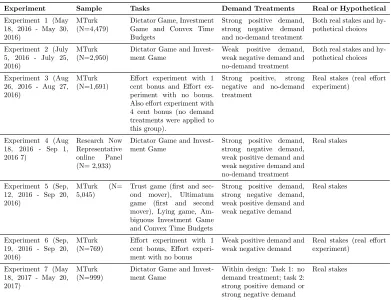
We conducted seven experiments in total to demonstrate our approach and to provide estimates of demand sensitivity on a wide range of standard experimental tasks (to save space, we provide citations for the tasks in web Appendix E). Our respondents complete one of eleven tasks: a dictator game; a risky investment game, without or with ambiguity; a convex time budget task; a trust game (first or second mover); an ultimatum game (first or second mover); a lying game; and a real e↵ort task with or without performance pay. We conduct all of our experiments online, primarily because the large number of treatments would be infeasible to implement in the laboratory. We designed the experiments to maxi-mize comparability. For all experiments except the e↵ort task, the action spaces are similar (they can be expressed as real numbers from 0 to 1); we pay the same show-up fee; recruit from the same participant pools; use the same mode of col-lection (online); the same response mode (sliders); and keep stakes as similar as possible.12
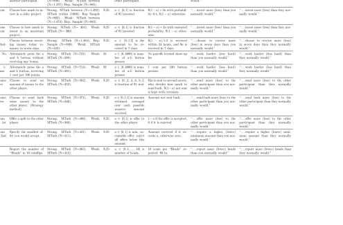
We employ two phrasings for our demand treatments. Our “weak” treatments explicitly tell participants that we expect high or low actions. For example, in the investment game, participants were told at the end of their instructions that “We expect that participants who are shown these instructions will invest more/less in the project than they normally would.”13 The strong treatments go further, telling participants that they will “do us a favor” by taking a higher or lower action. For example, in the dictator game, participants in the positive demand
12For the e↵ort task, we replicated the design employed in DellaVigna and Pope (2017) and DellaVigna and Pope (2018). The primary di↵erences with our other tasks are a higher show-up fee and a di↵erent response mode (e↵ort).
condition were told “You will do us a favor if you give more/less to the other participant than you normally would.” We keep the phrasing of the demand treatments as homogeneous as possible across tasks. In the two-player games we do not provide information about demand treatments shown to the other player, but our approach could be extended to create common knowledge about demand.
Table 6 summarizes the design features of each experiment, and Table 7 provides design details, parameters, and the exact wording of the demand treatments for each task. Figure A1 gives an example from the experimental interface. Full experimental instructions can be found on the journal webpage.
A. Participant populations
We conducted six experiments with approximately 16,000 participants (or “work-ers”) on Amazon Mechanical Turk (MTurk) (Experiments 1–3 and 5–7), and one experiment with around 3,000 participants using an online panel sample rep-resentative of the US population in terms of region, age, income, and gender (Experiment 4). MTurk is an online labor marketplace that is frequently used by researchers for surveys and experiments. It is attractive because it o↵ers a large and diverse pool of workers. There is some evidence that MTurk workers are more attentive to instructions than college students (Hauser and Schwarz, 2016). To participate in our MTurk experiments, workers had to live in the U.S, have an overall approval rating of more than 95 percent, and have completed more than 500 tasks on MTurk, fairly standard parameters in research on MTurk.14
Most workers on MTurk are experienced in taking surveys, which might a↵ect the external validity of our results. We used the representative sample, whose participants are less experienced with social science experiments, to replicate a subset of our findings. The sample is maintained by a market research company,
Research Now.
B. Pre-analysis plans
Our experiments were conducted in a sequence, between May 2016 and May 2017. Each is described in a pre-analysis plan (PAP) posted online prior to launch.15 The sequence is laid out in Table 6. For each experiment, the PAP details the data to be collected, treatment variables, experimental instructions, and how we planned to analyze that experiment’s data.
However, presenting the data experiment-by-experiment is repetitious. There-fore, for brevity and clarity of exposition, in the paper we pool the data and analyze all tasks side-by-side for our weak and strong demand treatments sepa-rately (this structure was described in pre-analysis plan 5). Our main analysis uses data from MTurk respondents with real stakes, which we have for all eleven tasks studied. In the analysis of heterogeneity we introduce hypothetical choice data from MTurk and the representative panel, which were collected for a subset of tasks. When averaging across tasks we weight observations to give equal weight to each task.
Other than this pooling across experiments, our analysis closely follows what was pre-specified.16 For completeness, web Appendix C presents all pre-specified
analyses, experiment-by-experiment. We refer to findings in the text if relevant.
C. Summary statistics
Tables D1 to D7 in the web Appendix present the pre-specified balance tables for all of the experiments. Tables D8 to D15 provide summary statistics on our respondents. Table D12 highlights that respondents from the online panel are representative of the US population by gender, income, age, and region, and other observables. Attrition was low, below 2 percent on average, and did not di↵er across demand treatment arms (Tables D16 and D17).
15The pre-analysis plans were posted on the Social Science Registry and can be found here: https://www.socialscienceregistry.org/trials/1248.
III. Applying the method
A. Bounding natural actions
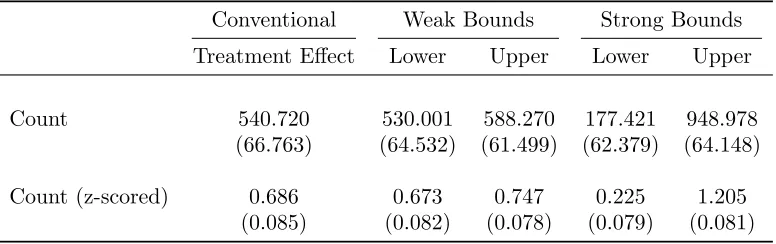
In this section we provide bounds on natural actions estimated using our weak and strong demand treatments. For a subset of tasks we also measured behavior with no demand treatment, and describe these results in Section IV.A where we discuss Monotonicity. Our objects of interest here are mean behavior in the positive (a+(⇣)) and negative (a (⇣)) demand conditions.
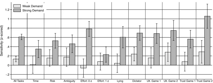
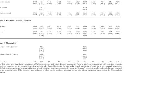
Panel A of Table 1 and Figure 2 show mean actions by task and demand treatment for incentivized MTurk respondents with weak treatments. Panel B of Table 1 and Figure 1 display sensitivities (a+(⇣) a (⇣)), in both raw and z-scored
units. Sensitivity is modest, averaging around 0.13 standard deviations, and frequently not significantly di↵erent from zero. The strongest responses (between 0.2–0.3 standard deviations) were observed for the dictator game, the ultimatum game second mover, and the trust game second mover. As we have argued, the weak manipulations seem likely to satisfy bounding for typical applications, so these results give cause for optimism.
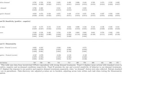
Panel A of Table 2 and Figure 2 show mean actions in the di↵erent demand treatment arms employing strong treatments. Panel B of Table 2 and Figure 1 display sensitivities. Behavior is responsive to our strong demand treatments, and sensitivity is significantly di↵erent from zero in all tasks, averaging around 0.6 standard deviations. Sensitivity is particularly high in the dictator game, for second movers in the trust and ultimatum games, and for unincentivized e↵ort. These manipulations are significantly stronger than likely implicit signals in most experiments or surveys, so providing quite conservative upper bounds on typical demand biases. However, they do demonstrate that participants are motivated to respond to signals about the researcher’s goals, and that responses can be significant when those signals are strong. Thus the attention researchers pay to potential demand e↵ects at the study design stage is well justified.
[Insert Table 1, Table 2, and Figures 1 and 2]
B. Bounding treatment e↵ects
10 minutes, earning one point per pair. One group were told that their score “will not a↵ect [their] payment,” while a second group received one cent per 100 points. By combining the bounds estimated for each incentive treatment we can construct bounds on the treatment e↵ect of performance pay on e↵ort provision.17 Table 3 displays the conventional treatment e↵ect (aL(1) aL(0), where “1” and
“0” correspond to the reward per 100 points), the upper bound of the treatment e↵ect (a+(1) a (0)), and the lower bound (a (1) a+(0)). In words, the lower bound on the treatment e↵ect is given by comparing participants who received performance pay, coupled with a negative demand treatment, to participants who received no performance pay, coupled with a positive demand treatment. We first show the bounds generated using our weak treatments, which are quite tight, ranging from 0.67 to 0.75 standardized units.18 The width of these bounds
corresponds to only 11 percent of the estimated treatment e↵ect (or 0.07 standard deviations), suggesting a limited role for experimenter demand in explaining the e↵ort response to incentives. Naturally, the bounds created using the more con-servative strong treatments are much wider, ranging from 0.23 to 1.21 standard deviations. Even these conservative bounds support the qualitative finding that e↵ort responds to incentives.
[Insert Table 3]
C. Confidence intervals
It is possible to compute confidence intervals for (a) the bounds themselves, and (b) the parameters contained by those bounds (a natural action or treatment e↵ect), following Imbens and Manski (2004) (see Appendix B.B7 for details). The latter can be thought of as “demand-robust” confidence intervals, combin-ing conventional parameter uncertainty due to samplcombin-ing error with the additional
17Our pre-analysis plans did not explicitly describe the bounding of treatment e↵ects, but it is an immediate extension of the approach to bounding actions.
18In constructing the bounds using our weak treatments we note that the average e↵ort in the no-incentive condition was actually slightly higher for those receiving negative demand than those receiv-ing positive demand, i.e. we observe a small monotonicity failure (a+(0) < a (0)). When sensitiv-ity is low, such outcomes can easily arise due to sampling variation; both values here are statisti-cally indistinguishable. In such cases, the procedure we propose in this section could lead to bounds on the treatment e↵ect with negative width. A conservative approach, which we follow, is to first “iron” the bounds on the no-incentive condition, by averaging them. Formally, one can compute
a+iron(⇣) = max{a+(⇣),0.5[a+(⇣) +a (⇣)]} anda
iron(⇣) = min{a (⇣),0.5[a+(⇣) +a (⇣)]}, and then use these values when computing the bounds on the treatment e↵ect, which becomea+(1) a
uncertainty about possible demand e↵ects. Uncertainty due to sampling error can be reduced in the usual way by increasing sample size (specifically, in the demand treatment arms), while uncertainty due to demand is reduced by select-ing minimally informative demand treatments, subject to Boundselect-ing (see section I.C). Table A3 presents confidence intervals computed from individual tasks us-ing both the weak and strong demand treatments. Table A4 presents confidence intervals on the bounds and treatment e↵ect of the e↵ect of incentive pay in the ef-fort experiment. Zero lies outside these confidence intervals, providing statistical support for the finding that incentives increased e↵ort.
D. Controlling for Demand
The nonparametric bounding approach described above yields bounds on treat-ment e↵ects, but researchers may be interested in point estimates that “control for” demand e↵ects. Intuitively, one might apply same-signed demand treatments (positive-positive or negative-negative) to the treatment group and the control group, with the goal of harmonizing demand between treatments. In this section we describe how using this approach can eliminate bias if demand treatments are assumed to be fully informative (pT = 1), and can reduce bias in other cases.
Derivations are given in web Appendix B.B8.19
We will assume throughout that Monotonicity holds strictly, i.e. >0 ( = 0 would imply no demand bias). The participant’s usual first-order condition, with demand treatment hT and optimal action a⇤(⇣, hT), is v1(a⇤(⇣, hT),⇣) +
(⇣)E[h|hT, hL(⇣)] = 0. A first-order Taylor approximation around the natural
actiona(⇣) yields:
a⇤(⇣, hT)⇡a(⇣) + (⇣)E[h|hT, hL(⇣)] (8)
where (⇣)⌘ (⇣)/v11(a(⇣),⇣) is a slope term capturing the e↵ect of beliefs on
actions, which we term “responsiveness.” is positive asv11<0.
Assume two treatment groups, ⇣ 2 {0,1}, with identical demand treatments
hT 2{ 1,1,;}, from which we estimate a treatment e↵ect a⇤(1, hT) a⇤(0, hT).
Its bias relative to the true e↵ect can be decomposed as follows:
Bias= [a⇤(1, hT) a⇤(0, hT)] [a(1) a(0)]
⇡ (1) E[h|hT, hL(1)] E[h|hT, hL(0)]
| {z }
Bias due to beliefs
+ ( (1) (0))E[h|hT, hL(0)]
| {z }
Bias due to “responsiveness”
The first term captures di↵erences in beliefs between the treatment and control environments, for example because they induce di↵erences in latent demand. The second captures di↵erences in behavioral responsiveness, given beliefs, for example because the treatment and control groups are at di↵erent locations on the cost of e↵ort function.20
Fully informative demand treatments
Importantly, in the special case where researchers are willing to assume that demand treatments are fully informative (pT = 1), we can eliminate the bias due
to beliefs: if hT is fully informative,E[h|hT, hL(1)] = E[h|hT, hL(0)] = 1 or 1.
We are left with the bias due to di↵erences in responsiveness. We can then ask whether this bias is important, by testing for di↵erences in sensitivity between treatment and control (an interaction e↵ect):21
[a⇤(1,1) a⇤(1, 1)]
| {z }
Sensitivity (⇣= 1)
[a⇤(0,1) a⇤(0, 1)]
| {z }
Sensitivity (⇣= 0)
⇡2 ( (1) (0)).
If this term is small, we can obtain a point estimate of the demand-free treatment e↵ect by comparing behavior on two same-signed demand treatment, essentially we are “controlling for” the influence of demand.
If sensitivity di↵ers significantly between treatment and control, we can still approximate the treatment e↵ect by averaging the estimates obtained with two
20In some settings it may be possible to sign the bias due to responsiveness. If demand treatments are applied, and bounding holds, the sign ofE[h|hT, hL(0)] is known and equal to the sign ofhT. Knowledge of the shape ofv can then help us to sign (1) (0). For example in the real e↵ort case, we expect responsiveness to decrease as e↵ort increases, due to the curvature of the cost of e↵ort function. That implies (1) (0)<0, in which case the bias due to responsiveness is negative when positive demand treatments are used.
positive and two negative demand treatments:
0.5 ([a⇤(1,1) a⇤(0,1)] + [a⇤(1, 1) a⇤(0, 1)])⇡a(1) a(0).
This approach is equivalent to estimating the treatment e↵ect from the midpoints of the bounds for the treatment and control groups. It relies on the symmetry of the first-order Taylor approximation.
Less informative treatments
Alternatively, researchers might wish to use same-signed weaker demand treat-ments to align beliefs among participants, without requiringpT = 1. In general this will not eliminate bias entirely, but we can derive conditions under which the bias will be reduced. Since di↵erences in responsiveness will no longer be testable we focus on the prospect of reducing the bias due to beliefs, which will be sufficient if variation in responsiveness between treatments is small.22 We find that when the latent demand biases have opposite signs (hL(1) = hL(0), which is the typical scenario that concerns researchers) our Bounding assumption is suf-ficient for two same-signed demand treatments to reduce the bias due to beliefs. When the latent demand biases have the same sign (hL(1) =hL(0)), same-signed demand treatments thatreinforce latent demand (i.e. hT =hL(1)) always reduce
bias. Sufficiently strong opposite-signed treatments reduce bias, but Bounding is not enough to guarantee this.
In summary, the Bounding assumption covers all cases except where the demand e↵ects in treatment and control agree with one another and disagree with the demand treatments used. To apply this approach, therefore, researchers may need to use judgment about the likely sign of demand e↵ects in their experiment, or report a range of estimates.
Applications
We apply the above-developed approaches to our e↵ort experiment in web Ap-pendix Table A1. For the strong demand treatments, where we have argued
pT = 1 is not an unreasonable assumption, we see large and statistically signif-icant di↵erences in sensitivity between the 0¢ and 1¢ treatment groups, so we
22In other words we ask when E[h|hT, hL(1)] E[h|hT, hL(0)] < E[h|hL(1)] E[h|hL(0)] , for
instead apply the “midpoint” technique. For the weak demand treatments we report treatment e↵ect estimates for both positive-positive and negative-negative demand treatment applications. Encouragingly, the estimates are all quite sim-ilar to one another, lying within 10 percent of the conventional treatment e↵ect estimate.
E. Structural estimates
Under further assumptions, strong demand treatments permit structural esti-mation of demand-free model parameters (v), as well as andE[h|hL]. Knowing
v allows the researcher to make predictions about behavior absent experimenter demand. Knowing allows them to quantify the importance of experimenter de-mand. Measuring beliefs can enable them to diagnose and eliminate the sources of latent demand e↵ects. We illustrate how structural estimation can be performed using the real e↵ort experiment. Because our model simply nests that of DellaV-igna and Pope (2018) (DP), we follow their approach to structural estimation.23
DP estimate the following utility function (expressed in our notation):
(9) v(a) = (s+⇣)a c(a)
The actionais e↵ort, measured in points on the task,sis an intrinsic motivation parameter (workers may exert e↵ort because they enjoy the task), andc(a) is a cost of e↵ort function. We assume the environment enters v only via the piece rate, so let⇣ 2{0,1,4}be a real number. DP solve the first order condition and estimate the model parameters using nonlinear least squares (NLLS).24
Adding demand to this utility function gives:
(10) U(a,⇣) = (s+⇣+ (⇣)E[h|hT, hL(⇣)])a c(a)
with corresponding first-order condition
(11) s+⇣+ (⇣)E[h|hT, hL(⇣)] c0(a⇤(⇣)) = 0
DP consider two alternative forms forc: First, a power functionc(a) =ka1+ /(1+ ), yielding optimal e↵ort equal to:
(12) a⇤(⇣) = ✓
s+⇣+ (⇣)E[h|hT, hL(⇣)]
k
◆1
Second, an exponential formc(a) =kexp( a)/ , with e↵ort level:
(13) a⇤(⇣) = 1log ✓
s+⇣+ (⇣)E[h|hT, hL(⇣)]
k
◆
We have seven treatment groups in total: neutral treatments with piece rates equal to 0 cents, 1 cent, and 4 cents per 100 points on the task; and positive and negative strong demand treatments in the 0 and 1 cent groups.25 Noting that E[h|hL(⇣)] =pL(⇣)hL(⇣) 2( 1,1), we can treat it as a single parameter whose sign identifieshL and whose magnitude identifies pL(⇣). This leaves us with 10 parameters: s, k, , (0), (1), (4), pL(0)hL(0), pL(1)hL(1), pL(4)hL(4), and
pT, so we need to impose some further restrictions.
First we assume that is fixed: (0) = (1) = (4) = , eliminating two parameters. In other words, varying incentives do not change the participants’ desire to please the experimenter. Second, as in the previous section, we assume
pT = 1, which implies thatE[h|hT, hL] =hT. By assumption this is not justified for our weak demand treatments, so we focus on the strong treatments. We are left with seven parameters, s, k, , , pL(0)hL(0), pL(1)hL(1), and pL(4)hL(4),
and are therefore exactly identified. We additionally estimate a specification in which we restrict latent demand to depend only on whether monetary incentives are present, i.e. pL(1)hL(1) =pL(4)hL(4).
While we use the same model as DP, identification comes from a di↵erent source. Under the assumption of no latent demand (as in DP), s, , and k
are identified from the three neutral treatment groups. When latent demand is present, the model parameters (s, ,k, ) are identified from thedemand treat-ment groups; with these in hand the neutral treatments allow us to back out the beliefspL(⇣)hL(⇣).
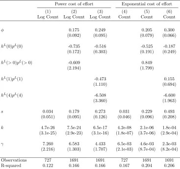
Full details of the estimation procedure, which follows DP, are provided in web Appendix B.B9. We estimate equation (12) in logs and equation (13) in levels.
timation results are presented in Table 4. Columns 1–3 correspond to the power cost function and columns 4–6 to the exponential cost function. In each case we first mirror DP by estimating s, , and k using only the neutral treatments, assuming that there is no latent demand.26 Second, we include all treatment groups and impose that latent demand depends only on whether monetary incen-tives are present (pL(1)hL(1) = pL(4)hL(4)). Third, we allow latent demand to di↵er across all three incentive levels. Coefficientssand are measured in cents per 100 points. Therefore,s= 1 is interpreted as intrinsic motivation playing an equivalent role to an incentive of 1 cent per 100 points.
Our main finding is a nontrivial preference for pleasing the experimenter. Our estimates of take values in the range 0.2–0.3 and are similar across specifications. A value of 0.2 implies that moving from complete uncertainty (E[h|hL] = 0) to complete certainty that high e↵ort is desired (E[h|hL] = 1) increases e↵ort as much as increasing the incentive by 0.2 cents per 100 points.
Our estimates of E[h|hL] are mostly negative, consistent with latent demand decreasing e↵ort. However, the estimates are noisy and typically not significantly di↵erent from zero. We estimate that in the 4 cent treatment,E[h|hL(4)]⇡ 6.5, while the theory requiresE[h|hL(4)]2( 1,1) (we note that the estimate is noisy and 1 lies well within the 95 percent confidence interval). This most likely reflects the fact that our demand treatments were only applied to the 0 and 1 cent treatment groups, so the e↵ort cost function must be extrapolated far out of sample to estimate beliefs for the 4 cent group. We provide further discussion on this point, and an illustrative figure, in web Appendix B.B9.
[Insert Table 4]
IV. Properties of demand e↵ects
In this section we examine some of the properties of demand e↵ects and the assumptions underlying our approach. We begin with a discussion of Monotonic-ity, examining whether it holds first on average and then at the individual level. Second we turn to the central mechanism that drives behavior in the model: changes in beliefs due signals about demand. Third, we consider the Bounding assumption. Although we cannot test it directly (since natural actions are not
observed), we show that our bounds seem reasonable given existing evidence on responsiveness to a particular design feature – anonymity in the dictator game – that has been argued to potentially induce variation in demand. Fourth, we study heterogeneity in sensitivity to our demand treatments, focusing on four dimen-sions: incentives, gender, attention, and participant pool. These are cases where we might expect our Monotone Sensitivity assumption to hold, such that vari-ation in sensitivity is informative about underlying varivari-ation in latent demand. Fifth, we examine the e↵ect of our demand treatments on the variance and full distribution of actions.
A. Monotonicity
Monotonicity on average
Our first theoretical assumption is Monotonicity: a+(⇣) aL(⇣) a (⇣). Panel C of Table 1 and Panel C of Table 2 examine this assumption for the subset of tasks in which we collected data without applying demand treatments.27 We estimate the following equation using the incentivized MTurk respondents, in whichP OSiandN EGiare dummy variables for the positive and negative demand
treatments, and the no-demand condition is the reference group:
ZYi=⇡0+⇡1P OSi+⇡2N EGi+"i
(14)
We find strong support for Monotonicity in average actions. The strong de-mand treatments always moved average actions in the intended direction, and in most cases the di↵erences are statistically significant. We find a significant nega-tive response to neganega-tive weak demand in the investment game and a significant positive response to weak positive demand in the dictator game. Responses to the the positive demand treatment in the investment game and the negative demand treatment in the dictator game have the wrong signs but are close to zero and not statistically significant. Finally, our data from the representative sample is fully consistent with Monotonicity for both the weak and strong treatments (see Table C18).
Testing monotonicity within-person
Our seventh experiment uses a within-participant design, collecting data on behavior first without, and then with a demand treatment. This allows us to examine Monotonicity directly at the individual level, and identify defiers, who try to do the opposite of the experimenters wishes. Intuitively, by observing who increases and who decreases their action in response to a positive demand treatment, we can identify who is a complier and who is a defier. As discussed in section I.D “too much” defiance can invalidate our bounds.
The design is as follows. MTurk participants were told that they would com-plete two tasks, and be paid according one of them, selected by chance. Half played the dictator game twice, and half the investment game twice. They first completed the task without any demand treatment, then again with the addition of a strong positive or negative demand treatment. We thus have four groups, split by dictator/investment game and positive/negative demand.
The model implies a simple interpretation of the data. Participants observe the first task, form a belief abouth, and make a choice. They then observe the second task with the demand treatment, update their belief, and make a new choice. Strict compliers, with >0, will increase their action relative to task 1, strict defiers with <0 will decrease it, and those with = 0 should take the same action in both tasks.28
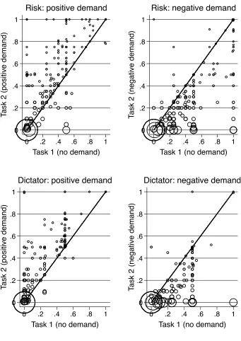
Our main findings are captured by Figure 3, which plots actions from tasks 1 and 2. In the positive demand treatments, strict compliers lie above the 45 degree line, strict defiers lie below and those who did not change their action lie on the line. Only about 5 percent of our respondents are strict defiers. About 30 percent do not change their behavior in response to our demand treatments, while the remaining 65 percent strictly comply with our demand treatments (proportions are similar across tasks). Thus we find very little evidence of defiance.
Table A2 presents mean actions and sensitivities estimated from the within design and the equivalent objects from the earlier between-participants
ments. For the within experiment, “no demand” cells are computed from task 1, while demand treatment cells and sensitivities from task 2. The sensitivities are quantitatively very similar in the between and within designs. This is en-couraging, as it suggests researchers can simply and cheaply obtain bounds using within-participant demand treatments, avoiding the need to recruit additional participants to apply our method.
Within-participant data can be used to construct “defier-corrected” bounds.29
These, with confidence intervals, are displayed in Table A6. They are almost identical to the conventional bounds, reflecting the low rate of defiance and giving further comfort that defiance is quantitatively unimportant. Table A5 reports raw actions separately for compliers and defiers.
B. Beliefs
The core mechanism in our model is that participants form beliefs about the experimenter’s objective in response to implicit or explicit signals. We examine this assumption with simple, unincentivized belief data collected after partici-pants had completed their experimental task. The purpose of the measures was a manipulation check, to ascertain that participants’ beliefs responded as expected to the demand treatments. We asked two questions: “What do you think is the result that the researchers of this study want to find?,” and “What do you think was the hypothesis of this research study?” Responses were binary: participants could respond that they thought the objective/hypothesis was either a high or low action.30 We assume that participants report a high belief if their posterior
(E[h|hL] or E[h|hT, hL]) is positive, and a low belief if negative, so the average
response tells us the fraction of participants with high beliefs.
Results for incentivized MTurk respondents are presented in Tables A8–A9 in the web Appendix. They confirm that our treatments moved average responses in the anticipated direction. Overall, the levels of beliefs and magnitudes of shifts in beliefs are similar for the strong and weak treatments, i.e. both were equally successful in fixing the sign of beliefs. In the theory, strong and weak treatments
are equally e↵ective at fixing the sign of beliefs ifpT pL, but stronger treatments lead to more extreme posteriors.31
C. Comparison of e↵ect sizes
Is the bounding assumption reasonable? Although it is not directly testable, we compare our bounds to previous manipulations that have been hypothesized to induce demand e↵ects. Our examples all come from the dictator game and include four studies that varied participants’ degree of anonymity, and a study in Sierra Leone that varied the presence of a white foreigner.32 We present e↵ect
sizes from these experiments and our own in Table A11.
Sensitivity to our weak treatments (a 17 percent reduction in giving under neg-ative versus positive demand) is very close to the average e↵ect size across these 5 studies (around 21 percent reduction in giving in response to treatment), and our strong treatments comfortably bound this average (a 42 percent reduction). Considering individual studies, our weak bounds are close in magnitude to those from Bolton, Katok and Zwick (1998), Barmettler, Fehr and Zehnder (2012), and Cilliers, Dube and Siddiqi (2015), but smaller than those from Ho↵man et al. (1994) and Ho↵man, McCabe and Smith (1996). These two studies in partic-ular, however, have been criticized for inducing potentially strong experimenter demand (Loewenstein, 1999), so may represent a scenario where the more conser-vative strong bounds are preferable. Their e↵ect sizes are close to or a bit larger than (and not significantly di↵erent from) our strong bounds.
The exercise is of course only suggestive, since responses in these studies include direct e↵ects of anonymity on behavior as well as potential experimenter demand. Additionally, the studies we consider were conducted in the laboratory and dif-fer in various other ways from our online setting. The results are nevertheless encouraging, in particular that our weak bounds seem to perform quite well.
31pT pLalso implies thatallparticipants’ beliefs should have the “correct” sign following a demand treatment. Not all of our participants reported correct beliefs following a demand treatment. This could be due to measurement error in our belief data, or, as we discuss in Appendix B.B3, participants might be inattentive to our demand treatments. If they are also inattentive to latent demand signals such participants do not threaten Bounding.
D. Heterogeneity
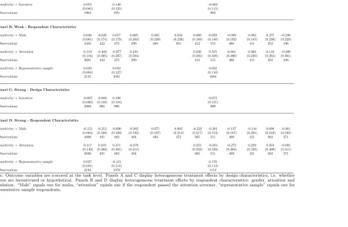
Does sensitivity to demand treatments vary by design and participant char-acteristics? Here, we examine heterogeneous responses to our strong and weak demand treatments on four pre-specified dimensions: by whether choices are in-centivized or hypothetical; gender; attentiveness; and participant pool (MTurk vs. representative online panel). Whether or not this heterogeneity can be inter-preted as informative about di↵erences in underlying latent demand depends upon whether Monotone Sensitivity holds for the environments under consideration, i.e. whether they belong to the same comparison class. We show in Appendix B.B3 that variation in incentives, attention, and the preference for pleasing the exper-imenter, (which may di↵er by gender or participant pool), form valid bases for comparison classes.
Incentivized vs. hypothetical choices
In MTurk experiments 1 and 2 we randomly assigned participants to make either hypothetical or incentivized choices. In theory, we would expect higher sensitivity in hypothetical choice, as the cost of deviating from the natural action is lower. To test this prediction, we regress standardized actions on a dummy,P OSi, taking
value one for the positive demand treatment and zero for the negative treatment; a dummy indicating incentivized choice,Mi; and their interaction:
ZYi = 0+ 1P OSi+ 2Mi⇥P OSi+ 3Mi+"i
(15)
Results for the weak and strong demand treatments are presented in Table 5. Interestingly, participants making hypothetical or incentivized choices responded very similarly to experimenter demand, in each task and on average, and if any-thing sensitivity is slightly higher when incentivized.
Relatedly, we ask how sensitivity di↵ers when we increase performance pay in the e↵ort task. Reasonable assumptions would imply sensitivity is decreasing in performance pay (see web Appendix B.B3). Table 2 shows that sensitivity to our strong treatments was around 3.5 times higher when e↵ort was unincentivized, as predicted. We do not see the same pattern under the weak treatments, though this may simply reflect the fact that sensitivity to these treatments was low.
One possibility is that our incentivized choices still involve relatively low stakes, and that we would see a di↵erence at higher stakes. Additionally, the theory allows to depend upon⇣ and another possibility is that raising the stakes also raises participants’ desire to please the experimenter (e.g. due to reciprocity). We see this as an interesting avenue for future work. Our results relate to previous work examining the e↵ects of incentives on behavior in the lab (Camerer et al., 1999).
Gender and attention
We measure self-reported gender in all tasks on MTurk and in the representative panel, and attentiveness in all tasks except the e↵ort task (since DP did not measure this variable). We define a participant as attentive if they passed an attention screener at the beginning of the task.33 We estimate the following
equation:
(16) ZYi= 0+ 1P OSi+ 2Hi+ 3Hi⇥P OSi+"i
whereHi is the dimension of heterogeneity of interest.
As can be seen in Table 5, we find that women respond more strongly to the strong demand treatments than men, with sensitivity around 0.15 standard devi-ations higher, but no significant di↵erence for the weak treatments (where overall sensitivity and thus statistical power is lower). We interpret the evidence as sug-gestive of greater desire to please the experimenter among women, which relates to the literature on gender di↵erences in preferences (Croson and Gneezy, 2009). Turning to attention, only 10 percent of MTurk respondents failed our screener, so we have little power to detect di↵erences in sensitivity. Table 5 shows higher sensitivity (around 0.12 standard deviations) to our weak and strong manipula-tions among attentive participants, but these e↵ects are not significant.34
33We use the screener developed by Berinsky, Margolis and Sances (2014). It presents participants with a paragraph of text that appears to direct them to select their preferred online news sources from a list, but concealed in the text is an instruction to instead choose two specific options. The assumption is that attentive respondents read the question and follow the concealed instruction, while inattentive respondents do not. Passing the attention check is weakly positively correlated with previous completion of MTurk tasks, so we also consider heterogeneity using a representative online panel whose respondents are generally less experienced and are unlikely to have seen the screener before. Moreover, there is little variation in sensitivity by experience, results are available on request.
In the representative online panel we find significantly higher sensitivity among women, and among attentive participants (see web Appendix C.C4). Approxi-mately 65 percent failed the screener, increasing our power here.
[Insert Table 5]
MTurk vs. representative online panel
Some researchers are concerned that MTurk workers are experienced research participants and may behave di↵erently than a more representative participant pool. In addition, MTurkers need to maintain a high work “acceptance” rating and may therefore be especially motivated to please the researcher (Berinsky, Huber and Lenz, 2012). To address such concerns, and to test an additional di-mension of heterogeneity, we replicated the MTurk dictator game and investment game experiments with respondents from a representative online panel, whose participants are less experienced in the types of tasks we consider. We used both weak and strong demand treatments, or no demand treatment. All choices were incentivized at the same stakes as in the MTurk experiments.35 Table 5 tests for
di↵erences in sensitivity between MTurk and representative survey participants, pooling tasks and for each task separately.36
Representative panel participants responded very similarly to MTurk partici-pants, with sensitivity on average 0.03 standard deviations higher (not significant) under both weak and strong treatments. There are some small di↵erences in sen-sitivity to the strong treatments at the game level (significant at 10 percent for the dictator game), but little evidence of systematic di↵erences between participant pools.
participants (p=0.10). Experiment 2 (weak treatments)finds slightly higher sensitivity for men (p=0.25) and attentive participants (p=0.53). Experiment 3 (e↵ort, strong treatments) finds almost identical sensitivity for men and women (p=0.95).
35Respondents in the online panel were incentivized with $1 stakes in the panel currency, which they can use to buy products in the survey provider’s online store. We discovered after the study that, while some of the products in the store have a value equivalent to $1, others have lower value. This means that the e↵ective stake size in the representative online panel may have been lower than on MTurk. Since we find no di↵erences in response to demand treatments depending on whether choices are incentivized or hypothetical on MTurk, we do not expect this to be an important concern.