An Error Correction Model for Forecasting Philippine Aggregate Electricity Consumption

An Error Correction Model for

Forecasting Philippine Aggregate

Electricity Consumption

Danao, Rolando and Ducanes, Geoffrey

University of the Philippines

2016

Online at

https://mpra.ub.uni-muenchen.de/87722/

Working Paper 2016-05R _{March 2017}

An Error Correction Model

for Forecasting Philippine

Aggregate Electricity

Consumption

By

Rolando A. Danao and Geoffrey M. Ducanes

University of the Philippines (UP) and

Energy Policy and Development Program (EPDP)

EPDP Working Papers are preliminary versions disseminated to elicit critical comments. They are protected by Republic Act No. 8293 and are not for quotation or reprinting without prior approval. This study is made possible by the generous support of the American People through the United States Agency for International Development (USAID) under the Energy Policy and Development Program (EPDP). EPDP is a four-year program implemented by the UPecon Foundation, Inc. The contents or opinions expressed in this paper are the authors’ sole responsibility and do not necessarily reflect the views of USAID or the United States Government or the UPecon Foundation, Inc. Any errors of commission or omission are the authors’ and should not be attributed to any of the above.

Rolando A. Danao1 _{and Geoffrey M. Ducanes}2

Abstract

This paper presents an error correction model for forecasting electricity consumption in the Philippines based on income, price, and temperature. The empirical evidence shows that there is a long-run positive and inelastic relationship between electricity consumption and income. We find that income, price, and temperature have significant short-run effects. Short-run demand is positive and inelastic with respect to income, negative and inelastic with respect to price, and positive and elastic with respect to temperature. Despite the small sample size, the model passes the standard diagnostic and parameter stability tests and performs well in within-sample and out-of-sample forecasting. It can be used not only for forecasting but also for analyzing, through simulations, the impacts on electricity consumption of changes in income, price, and temperature.

The simulations confirm that, in the long run, electricity consumption is mainly driven by economic growth. Increasing GDP growth rate from 6% per year to 7% could increase electricity consumption at the end of 15 years by 10%. Although the effect of electricity price on electricity consumption is small (because of low price elasticity in absolute terms) and the effect of temperature change is also small (because annual average temperature change is small), their combined effects could add up and our simulation indicates that under very conservative assumptions, electricity consumption at the end of 15 years could rise further by 2%. Thus, it is important to include these variables in the simulations in order to account for their combined effects.

JEL Classification: C53

Key words: Electricity consumption, forecasting, error correction model

This study is made possible by the generous support of the American People through the United States Agency for International Development (USAID) under the Energy Policy and Development Program (EPDP). EPDP is a four-year Program implemented by the UPecon Foundation, Inc. The contents or opinions expressed in this paper are the authors’ sole responsibility and do not necessarily reflect the views of USAID or the United States Government or the UPecon Foundation, Inc. Any errors of commission or omission are the authors’ and should not be attributed to any of the above.

AN ERROR CORRECTION MODEL FOR FORECASTING PHILIPPINE AGGREGATE ELECTRICITY CONSUMPTION

1. Introduction

Electricity is linked to practically all aspects of national development (industrial production, agricultural production, education, health, etc.) that forecasting the country’s future electricity demand has become crucial to energy planning and management. Government planners rely on sound and reliable electricity demand projections in their development planning and forecasts that are way out of line can have serious economic consequences. The objective of this study is to develop a forecasting model for aggregate electricity demand in the Philippines. Specifically, we develop an error correction model

(ECM) where electricity demand is related to economic and climatic variables. We believe this is the first time an error correction model is used for forecasting electricity consumption in the Philippines. It is also the first time that a Philippine model for electricity consumption includes temperature as an explanatory variable.

2. Demand for Electricity

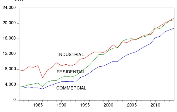
Table 2.1. Electricity Consumption by Type of Use: Philippines, 1981 and 2014

1981 2014 Annual Growth Rate (%) GWh % Share GWh % Share 1981-2014 Total Consumption 18,583 100 77,261 100 4.41

Type of Use

Industrial 7,597 40.88 21,429 27.74 3.19 Residential 3,424 18.42 20,969 27.14 5.65 Commercial 3,157 16.99 18,761 24.28 5.55 Power Loss 2,150 11.57 7,270 9.41 3.76 Utilities Own Use 1,157 6.23 6,646 8.60 5.44 Others 1,098 5.91 2,186 2.83 2.11

Source: Philippine Statistical Yearbook, 2014

Figure 2.1. Electricity consumption (GWh) by type of use, Philippines: 1981-2014

0 4,000 8,000 12,000 16,000 20,000 24,000

1985 1990 1995 2000 2005 2010 GW h

INDUSTRIAL

COMMERCIAL RESIDENTIAL

Table 2.2. Access to Electricity (% of population)

Year Rural Urban All

1990 46.4 84.0 65.4

2000 51.9 91.0 71.3

2010 72.8 94.4 83.3

Source: Index mundi, sourced from World Bank Sustainable Energy for All, Global Electrification data base.

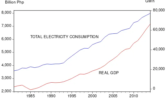
The evolution of electricity consumption in the Philippines is closely related to that of real gross domestic product (see Figure 2.2). In fact, the correlation coefficient between these two variables is 0.98. This strong positive relationship is graphically shown in Figure 2.3. But in terms of growth rates, electricity consumption outpaced real GDP by a factor of 1.3. (The average annual growth rate of real GDP for the period 1981-2014 was 3.42%.)

Figure 2.2. Total electricity consumption (GWh) and real gross domestic product (billion pesos at 2000 constant prices), Philippines: 1981-2014

2,000 3,000 4,000 5,000 6,000 7,000 8,000 0 20,000 40,000 60,000 80,000

1985 1990 1995 2000 2005 2010 REAL GDP TOTAL ELECTRICITY CONSUMPTION

Billion Php GW h

Figure 2.3. Total electricity consumption vs real gross domestic product

10,000 20,000 30,000 40,000 50,000 60,000 70,000 80,000

2,000 3,000 4,000 5,000 6,000 7,000 8,000 REAL GDP (Billion Php)

3. Model Framework

From the point of view of economic theory, demand for electricity is a function of income and price of electricity. In recent years, an increasing number of researchers have included weather variables among the factors affecting electricity consumption (Lam et al. [2008]; Zachariadis [2010]; Goel and Goel [2014]). Obviously, climate change such as increasing temperature will increase electricity demand related to cooling requirements.

We begin with a basic relationship between electricity consumption (𝑦𝑦) and real gross domestic product (𝑥𝑥) and electricity price (𝑝𝑝) given as an autoregressive distributed lag (ARDL) model,

𝑦𝑦𝑡𝑡 =𝛽𝛽0+𝛽𝛽1𝑥𝑥𝑡𝑡+𝛽𝛽2𝑥𝑥𝑡𝑡−1+𝛽𝛽3𝑝𝑝𝑡𝑡+𝛽𝛽4𝑝𝑝𝑡𝑡−1+𝛽𝛽5𝑦𝑦𝑡𝑡−1+ 𝜀𝜀𝑡𝑡 (3.1)

where 𝑦𝑦_𝑡𝑡, 𝑥𝑥_𝑡𝑡, and 𝑝𝑝_𝑡𝑡 are in natural logarithms and, for stability, |𝛽𝛽₅| < 1. (We follow the convention that lower case italics denote variables in natural logarithms.) In long-run equilibrium, 𝑦𝑦_𝑡𝑡 =𝑦𝑦_𝑡𝑡−1, 𝑥𝑥_𝑡𝑡 =𝑥𝑥_𝑡𝑡−1, and 𝑝𝑝_𝑡𝑡 =𝑝𝑝_𝑡𝑡−1. Hence, from (3.1),

(1− 𝛽𝛽₅)𝑦𝑦_𝑡𝑡 =𝛽𝛽₀+ (𝛽𝛽₁+𝛽𝛽₂)𝑥𝑥_𝑡𝑡+ (𝛽𝛽₃+𝛽𝛽₄)𝑝𝑝_𝑡𝑡+𝜀𝜀_𝑡𝑡 (3.2)

Thus, the long-run equation is

𝑦𝑦𝑡𝑡 =_{1− 𝛽𝛽}𝛽𝛽0 5+

𝛽𝛽1+𝛽𝛽2

1− 𝛽𝛽₅ 𝑥𝑥𝑡𝑡+

𝛽𝛽3+𝛽𝛽4

1− 𝛽𝛽₅ 𝑝𝑝𝑡𝑡+𝑢𝑢𝑡𝑡 (3.3)

where 𝑢𝑢_𝑡𝑡= 𝜀𝜀𝑡𝑡

1−𝛽𝛽5. The short-run dynamics is introduced by subtracting 𝑦𝑦𝑡𝑡−1 from both sides

of (3.1) and adding and subtracting 𝛽𝛽₁𝑥𝑥_𝑡𝑡−1 and 𝛽𝛽₃𝑝𝑝_𝑡𝑡−1 on the right-hand side, resulting in the following equation:

∆𝑦𝑦𝑡𝑡 =𝛽𝛽1∆𝑥𝑥𝑡𝑡+𝛽𝛽3∆𝑝𝑝𝑡𝑡+ (𝛽𝛽5−1)�𝑦𝑦𝑡𝑡−1−_{1− 𝛽𝛽}𝛽𝛽0 5−

𝛽𝛽1+𝛽𝛽2

1− 𝛽𝛽₅ 𝑥𝑥𝑡𝑡−1−

𝛽𝛽3+𝛽𝛽4

1− 𝛽𝛽₅ 𝑝𝑝𝑡𝑡−1�+𝜀𝜀𝑡𝑡 (3.4)

4. ECM Empirical Specification and Data for an Annual Model

Specifying an electricity demand function is complicated by the existence of block pricing in some distribution utilities in which prices differ in each block. From economic theory, the appropriate price variable is marginal price. But Taylor [1975] argued that to use only the marginal price in this case neglects the income effect of the intramarginal prices and introduces biases in the parameter estimates. However, Berndt [1984] estimated these biases and found them to be negligible.

At a highly aggregated level of data (national level), electricity consumption under differing block pricing structures make it impossible to determine marginal price. Thus, as a measure of electricity price, we use the ex post average price, computed as total expenditure on electricity divided by total kilowatt hours consumed. Van Helden et al. [1987] estimated residential electricity demand functions using different price variables and found support for using average price in the demand function for electricity.

In the empirical specification of the ECM, the practice is to include other exogenous variables and allow a richer dynamic structure by including lags of the short-run terms. However, since the number of lags to include is unknown, it has to be empirically determined and the suggested procedure is to “test down” the lagged terms and produce a parsimonious model without violating the usual diagnostic tests.

In addition to real GDP and electricity price, we include temperature as an exogenous variable that affects electricity consumption in the short run. Thus, the variables used in the model are (a) total electricity consumption (Y, in GWh), (b) real gross domestic product (X, in 2000 pesos), (c) real electricity price (P, in 2000 pesos/KWh), and

temperature (Z, in degrees Celsius). Real gross domestic product data was obtained from

the Philippine Statistical Authority, total electricity consumption was obtained from the

Department of Energy, and temperature was obtained from the Climate Research Unit of the

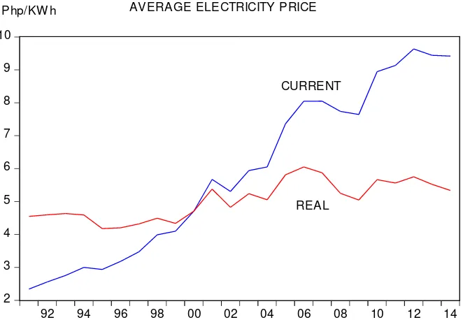
University of East Anglia (graph of temperature is shown in Figure 4.1). Meralco average

price was used as a proxy for electricity price. Meralco is the largest distribution utility,

accounting for 55%-60% of total electricity sales during the last decade. Figure 4.2 shows

the movement of the current and real prices, where the latter was obtained by using the

Figure 4.1. Temperature

25.8 26.0 26.2 26.4 26.6 26.8 27.0

92 94 96 98 00 02 04 06 08 10 12 14

Degrees Celsius AVERAGE ANNUAL TEMPERATURE

Source of basic data: Climate Research Unit, University of East Anglia

Figure 4.2. Electricity Price

2 3 4 5 6 7 8 9 10

92 94 96 98 00 02 04 06 08 10 12 14 Php/KW h AVERAGE ELECTRICITY PRICE

CURRENT

REAL

Source of basic data: Current price provided by Meralco. Real price obtained by deflating current price

Unit Root Tests and Cointegration

Error-correction modeling requires determining the order of integration of each

variable and is done by testing for the presence of a unit root. If a series has a unit root and

its first difference is stationary or I(0), the series is integrated of order 1 or I(1). Testing for

a unit root may be accomplished by using the Augmented Dickey-Fuller (ADF) Test (Dickey

and Fuller [1979]). The null hypothesis in an ADF test is that the series under consideration

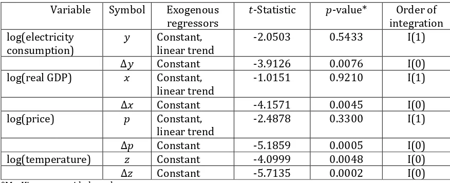
has a unit root. The ADF tests showed that 𝑦𝑦_𝑡𝑡,𝑥𝑥_𝑡𝑡, and 𝑝𝑝_𝑡𝑡 are I(1) while 𝑧𝑧_𝑡𝑡 is I(0) (Table 4.1).

Table 4.1. Summary of ADF Tests

Variable Symbol Exogenous regressors

𝑡𝑡-Statistic 𝑝𝑝-value* Order of integration

log(electricity consumption)

𝑦𝑦 Constant, linear trend

-2.0503 0.5433 I(1)

∆𝑦𝑦 Constant -3.9126 0.0076 I(0)

log(real GDP) 𝑥𝑥 Constant, linear trend

-1.0151 0.9210 I(1)

∆𝑥𝑥 Constant -4.1571 0.0045 I(0)

log(price) 𝑝𝑝 Constant,

linear trend

-2.4878 0.3300 I(1)

∆𝑝𝑝 Constant -5.1859 0.0005 I(0)

log(temperature) 𝑧𝑧 Constant -4.0999 0.0048 I(0)

∆𝑧𝑧 Constant -5.7135 0.0002 I(0)

*MacKinnon one-sided 𝑝𝑝-value.

The next step is to determine if the economic variables, which are all I(1), are

cointegrated, i.e., there is a long-run relationship among them given by the equation

(cointegrating equation)

𝑦𝑦𝑡𝑡 =𝛽𝛽0+𝛽𝛽1𝑥𝑥𝑡𝑡+𝛽𝛽2𝑝𝑝𝑡𝑡+𝜀𝜀𝑡𝑡 (4.1)

where 𝜀𝜀_𝑡𝑡 is the error term. A number of cointegration tests are available including the residual-based Engle-Granger [1987] test, the Hansen [1992] parameter instability test, and

the error correction test (Enders [2010]; Kremers et al. [1992]). Although the

Engle-Granger test is popular, it has some problems such as the common factor restrictions

problem, its low power, and small sample bias (Harris [1995]). Hansen’s test is based on the

notion that parameter instability arises when there is no cointegration. It is implemented by

estimating the cointegrating equation by the Fully Modified Ordinary Least Squares

(FMOLS) procedure [Phillips and Hansen [1990]). The error correction test, suggested by

term is equal to zero. If the null hypothesis is true, then there is no cointegration; otherwise,

cointegration is indicated.3 _{Kremers et al. [1992] showed that this test is more powerful}

than the Augmented Dickey-Fuller test because no common factor restrictions are imposed.

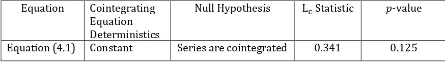
Equation (4.1) was estimated using the COINTREG command in EViews 9 and the

result is presented in Table 4.2. The Hansen cointegration test is shown in Table 4.3. With a

𝑝𝑝-value of 0.125, the null hypothesis of cointegration cannot be rejected.

Table 4.2. Estimation output for equation (4.1)

Dependent variable: 𝑦𝑦

Coefficient Std. Error 𝑡𝑡-Statistic 𝑝𝑝-value

𝑥𝑥 0.959 0.119 8.028 0.0000

𝑝𝑝 0.258 0.295 0.874 0.3930

constant 2.389 0.7001 3.409 0.0029

𝑅𝑅2_{= 0.94}

Table 4.3. Cointegration Test – Hansen Parameter Instability

Equation Cointegrating Equation Deterministics

Null Hypothesis L_c Statistic 𝑝𝑝-value

Equation (4.1) Constant Series are cointegrated 0.341 0.125

Although the variables are cointegrated, electricity price 𝑝𝑝 has a positive sign. As

this does not conform to economic theory, the price variable was dropped from equation

(4.1) resulting in the potential long-run relationship between electricity consumption and

real gross domestic product:

𝑦𝑦𝑡𝑡 =𝛽𝛽0+𝛽𝛽1𝑥𝑥𝑡𝑡+𝑢𝑢𝑡𝑡 (4.2)

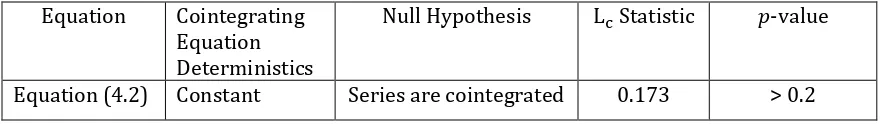
This new cointegrating equation was estimated by COINTREG; the regression output is

shown in Table 4.4 and the Hansen cointegration test result presented in Table 4.5. With a

𝑝𝑝-value greater than 0.2, we cannot reject the null hypothesis that the variables 𝑦𝑦 and 𝑥𝑥 are cointegrated. This result is confirmed in the next section where it is shown that these two

variables have an error correction representation, a necessary and sufficient condition for

cointegration by virtue of the Granger representation theorem.

3

Table 4.4. Estimation output for equation (4.2)

Dependent variable: 𝑦𝑦

Coefficient Std. Error 𝑡𝑡-Statistic 𝑝𝑝-value

𝑥𝑥 1.014 0.174 5.842 0.0000

constant 2.343 1.452 1.614 0.1223

𝑅𝑅2_{= 0.94}

Table 4.5. Cointegration Test – Hansen Parameter Instability

Equation Cointegrating Equation Deterministics

Null Hypothesis L_c Statistic 𝑝𝑝-value

Equation (4.2) Constant Series are cointegrated 0.173 > 0.2

5.

Estimation of the ECM and Statistical Tests

With the long-run relationship in equation (4.2), we specify an Error Correction

Model that captures the short-run dynamics involving not only the short-run effects of real

GDP but also of electricity price and temperature. After experimenting with different lag

structures, we came up with the following single-equation ECM:

ECM1: ∆𝑦𝑦_𝑡𝑡 =𝛼𝛼₁∆𝑥𝑥_𝑡𝑡+𝛼𝛼₂∆𝑝𝑝_𝑡𝑡−1+𝛼𝛼₃∆𝑧𝑧_𝑡𝑡+𝜆𝜆(𝑦𝑦_𝑡𝑡−1− 𝛽𝛽₀− 𝛽𝛽₁𝑥𝑥_𝑡𝑡−1) +𝑣𝑣_𝑡𝑡 (5.1)

We note that the single-equation ECM can be used only when the cointegrating vector is

unique and the variables on the right-hand side are weakly exogenous (Harris [1995]). The

uniqueness of the cointegrating vector follows from the fact that the cointegrating equation

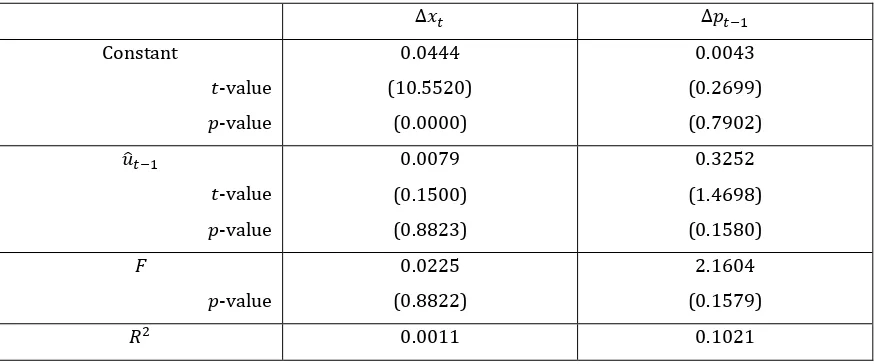
has only two variables. Weak exogeneity is established by showing that ∆𝑥𝑥_𝑡𝑡, ∆𝑝𝑝_𝑡𝑡−1 and ∆𝑧𝑧_𝑡𝑡 do not depend on the long-run disequilibrium represented by 𝑢𝑢�_𝑡𝑡−1 in equation (4.2) (Harris [1995], Enders [2010]):

𝑢𝑢�𝑡𝑡−1 =𝑦𝑦𝑡𝑡−1− 𝛽𝛽̂0− 𝛽𝛽̂1𝑥𝑥𝑡𝑡−1

Obviously, temperature does not depend on the disequilibrium but we need to test the weak

using the 𝑡𝑡-test. The 𝑡𝑡-test is applicable since the variables in the regression are I(0). The

results of the tests are reported in Table 5.1.

Table 5.1. Tests of Weak Exogeneity

∆𝑥𝑥𝑡𝑡 ∆𝑝𝑝𝑡𝑡−1

Constant

𝑡𝑡-value

𝑝𝑝-value

0.0444

(10.5520)

(0.0000)

0.0043

(0.2699)

(0.7902)

𝑢𝑢�𝑡𝑡−1

𝑡𝑡-value

𝑝𝑝-value

0.0079

(0.1500)

(0.8823)

0.3252

(1.4698)

(0.1580)

F

𝑝𝑝-value

0.0225

(0.8822)

2.1604

(0.1579)

𝑅𝑅2 _{0.0011 0.1021}

The test equations in Table 5.1 pass the standard diagnostic tests. Since the coefficients of

𝑢𝑢�𝑡𝑡−1 are not significantly different from zero, we conclude that real gross domestic product

and electricity price are weakly exogenous.

Model (5.1) may be estimated by the two-step residual-based Engle-Granger

method (Harris [1995]) but the recommended approach is to estimate the long-run

relationship jointly with the short-run dynamics as given in model (5.1). This approach is

preferred because estimating the cointegrating equation (4.2) separately results in

considerable small-sample bias (Kennedy [2003]; Banerjee et al. [1993]; Inder [1993]).

Moreover, Bewley [1979] showed that simultaneous estimation results in more efficient

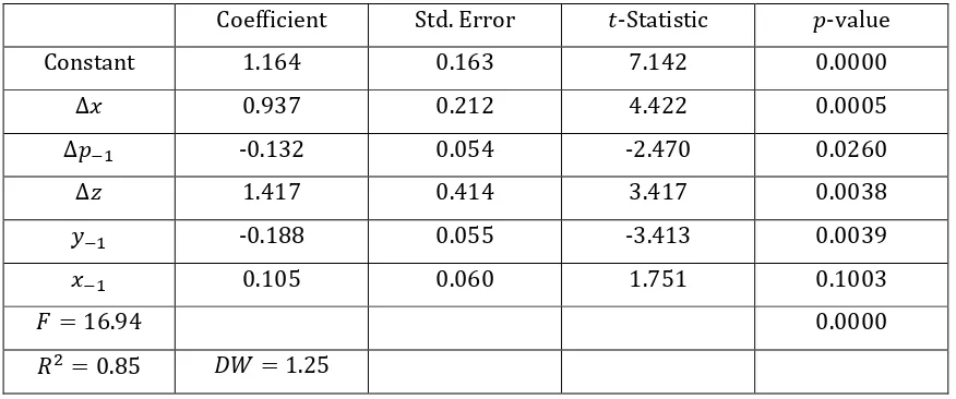
estimates of the long-run parameter. To estimate model (5.1), we rewrite it as

∆𝑦𝑦𝑡𝑡 =𝛼𝛼0+𝛼𝛼1∆𝑥𝑥𝑡𝑡+𝛼𝛼2∆𝑝𝑝𝑡𝑡−1+𝛼𝛼3𝑧𝑧𝑡𝑡+𝜆𝜆𝑦𝑦𝑡𝑡−1+𝛾𝛾𝑥𝑥𝑡𝑡−1+𝜈𝜈𝑡𝑡 (5.2)

Table 5.2. Estimated ECM1: Annual Electricity Consumption Dependent variable: ∆𝑦𝑦

Coefficient Std. Error 𝑡𝑡-Statistic 𝑝𝑝-value

Constant 1.164 0.163 7.142 0.0000

∆𝑥𝑥 0.937 0.212 4.422 0.0005

∆𝑝𝑝−1 -0.132 0.054 -2.470 0.0260

∆𝑧𝑧 1.417 0.414 3.417 0.0038

𝑦𝑦−1 -0.188 0.055 -3.413 0.0039

𝑥𝑥−1 0.105 0.060 1.751 0.1003

𝐹𝐹= 16.94 0.0000

𝑅𝑅2_{= 0.85 𝐷𝐷𝐷𝐷= 1.25}

The estimated equation passes Ramsey’s RESET test for specification error,

Breusch-Godfrey Serial Correlation LM Test, Breusch-Pagan-Breusch-Godfrey Heteroskedasticity Test, the

Jarque-Bera Normality of Residuals Test, the CUSUM Test and the CUSUM of Squares Test

for parameter stability (Vogelgang [2005])4_{. A summary of these test results is given in}

Table 5.3 and in Figure 5.1 and Figure 5.2.

Table 5.3. Summary of Statistical Diagnostic Tests for ECM1 (Table 5.2)

Test H₀ Statistic 𝑝𝑝-value

Ramsey’s RESET No specification error 0.6625 0.4293

Breusch-Godfrey Serial Correlation LM Test

No serial correlation 5.6834 0.1280

Breusch-Pagan-Godfrey Heteroskedasticity Test

No heteroskedasticity 4.9300 0.4245

Jarque-Bera Normality Test Normal residuals 0.2916 0.8643

Figure 5.1. The CUSUM TEST

The graph of the CUSUM Test statistic is inside the 5% significance level bounds; hence, the parameters are stable.

-12 -8 -4 0 4 8 12

00 01 02 03 04 05 06 07 08 09 10 11 12 13 14

CUSUM 5% Significance

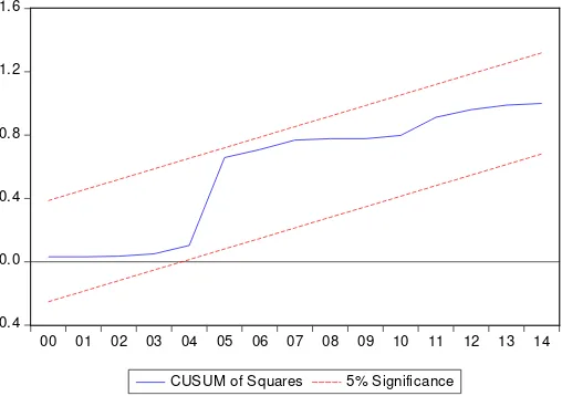
Figure 5.2. CUSUM OF SQUARES TEST

The graph of the CUSUM of Squares Test statistic is inside the 5% significance level band; hence, the parameters are stable.

-0.4 0.0 0.4 0.8 1.2 1.6

00 01 02 03 04 05 06 07 08 09 10 11 12 13 14

CUSUM of Squares 5% Significance

The estimated equation is written in ECM equation form (5.1) as

∆𝑦𝑦𝑡𝑡 = 0.937∆𝑥𝑥𝑡𝑡−0.132∆𝑝𝑝𝑡𝑡−1+ 1.417∆𝑧𝑧𝑡𝑡−0.188(𝑦𝑦𝑡𝑡−1−6.191−0.558𝑥𝑥𝑡𝑡−1) (5.3)

have significant negative effects. The speed of adjustment, denoted by 𝜆𝜆 in equation (5.1) and whose estimate is −0.188, has the correct sign in accordance with convergence toward long-run equilibrium. Moreover, it is significantly different from zero, indicating that an error correction representation exists, thereby confirming, by the Granger Representation Theorem, the earlier result that electricity consumption and GDP are cointegrated. It says that about 19% of the discrepancy between actual and equilibrium value of electricity consumption is corrected every year.

The short-run price elasticity of −0.13 is significant and conforms to the common finding that in the short run, electricity demand has a low sensitivity to price (Zachariadis [2010]; Galindo [2005]; Hunt and Manning [1989]; Bianco et al. [2010]).

The model estimates a short-run income elasticity of 0.94 which is higher than the estimated long-run income elasticity of 0.105/0.188 = 0.56. This result, where short-run income elasticity is higher than long-run income elasticity, has also been observed in other countries (Hunt and Manning [1989] for UK and Amarawickrama and Hunt [2008] for Sri Lanka). They argued that an increase in income causes “an immediate increase in derived demand for energy in the short-term, but this derived demand is reduced in the longer-term as more energy efficient machines are installed” (Hunt and Manning [1989]). In the Philippines, some indication of energy efficiency can be observed during the period 2003-2014, coinciding with the second half of the estimation period. Energy efficiency may be measured by energy intensity, defined as electricity consumption per unit of output. Energy intensity steadily declined from 13.21 GWh/billion pesos in 2003 to 10.78 GWh/billion pesos in 2014 or an average decline of 1.8% per year. This suggests that, during the 2003-2014, the Philippines was producing more output with less energy.

6.

Model Forecasting Performance

The forecasting performance of models is usually measured by the accuracy of the model’s forecasts. The most widely used measure of accuracy is the mean absolute percent error (MAPE)5 _{which has the advantage of being dimensionless. The estimated model}

performed well in historical simulation with an MAPE of 1.47%. In addition, the Theil inequality coefficient of 0.009 is close to zero, where zero indicates a perfect forecast

5_{MAPE =}1

𝑇𝑇∑ � 𝑦𝑦𝑡𝑡−𝑦𝑦�𝑡𝑡

𝑦𝑦𝑡𝑡 �× 100 𝑇𝑇

𝑡𝑡=1 , where 𝑦𝑦𝑡𝑡 is the actual value of the dependent variable and 𝑦𝑦�𝑡𝑡 is the predicted

(Vogelvang [2005]). The actual and forecasted electricity consumptions for the estimation period are graphically shown in Figure 6.1.

Figure 6.1. Historical Simulation: 1992-2014

20,000 30,000 40,000 50,000 60,000 70,000 80,000

92 94 96 98 00 02 04 06 08 10 12 14 GW h TOTAL ELECTRICITY CONSUMPTION

ACTUAL

FORECAST

Out-of-Sample Forecast Performance

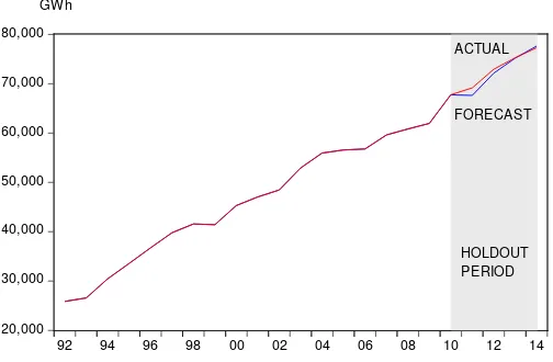
Besides model performance “within-sample”, as was done above, the model is also tested “out-of-sample”, where forecasts are made ex post (i.e., forecasts for which actual values are known but are outside the estimation period). For this purpose, the model was reestimated over the sample period 1992-2010, making 2011-2014 the holdout period. The reestimated model’s forecast in the holdout period had an MAPE of 0.97% and a Theil inequality coefficient of 0.006. These results validate the within-sample performance of the model. The graphs of the out-of-sample forecast together with the actual values are shown in Figure 6.2.

Figure 6.2. Out-of-Sample Forecast

20,000 30,000 40,000 50,000 60,000 70,000 80,000

92 94 96 98 00 02 04 06 08 10 12 14 ACTUAL

FORECAST

A Comparison with Other Models

It would be interesting to see if the presence of drivers of electricity consumption other than GDP, as in ECM1, improves the forecasting ability of the error correction model. So we construct another ECM, denoted as ECM2, with real GDP as the only explanatory variable. We also present the forecasting performance of an elasticity-based model (where elasticity is the elasticity of electricity consumption with respect to real GDP). This is a commonly used forecasting method in the absence of an econometrically developed model because it is simple, can be done quickly, and does not require a sophisticated forecaster to implement. These models are presented below.

(a) ECM2: ECM with GDP as the only explanatory variable Table 6.1. Estimation of ECM2

Dependent variable: ∆𝑦𝑦

Coefficient Std. Error 𝑡𝑡-Statistic 𝑝𝑝-value

Constant 0.927 0.226 4.095 0.0007

∆𝑥𝑥 1.002 0.340 2.949 0.0086

𝑦𝑦−1 -0.133 0.075 -1.783 0.0914

𝑥𝑥−1 0.062 0.085 0.727 0.4764

𝐹𝐹 = 6.35 0.0040

𝑅𝑅2_{= 0.51 𝐷𝐷𝐷𝐷= 2.20}

(b)Elasticity-based model

In income elasticity-based forecasting we use the following definition of income elasticity of demand (𝜂𝜂_𝑡𝑡):

𝜂𝜂𝑡𝑡 =

(𝑌𝑌_𝑡𝑡− 𝑌𝑌_𝑡𝑡−1)/𝑌𝑌_𝑡𝑡−1 (𝑋𝑋_𝑡𝑡− 𝑋𝑋_𝑡𝑡−1)/𝑋𝑋_𝑡𝑡−1,

where 𝑌𝑌_𝑡𝑡 is total electricity consumption and 𝑋𝑋_𝑡𝑡 is real GDP. Solving for 𝑌𝑌_𝑡𝑡, we get

𝑌𝑌𝑡𝑡 =𝑌𝑌𝑡𝑡−1�𝜂𝜂𝑡𝑡𝑋𝑋𝑡𝑡_𝑋𝑋− 𝑋𝑋𝑡𝑡−1

A historical value of 𝜂𝜂 is obtained and assumed to remain constant in the forecast horizon.

𝑌𝑌𝑡𝑡 is forecast given a starting value 𝑌𝑌0 and the assumed values of 𝑋𝑋𝑡𝑡 in the forecast horizon.

For our purpose, we use 𝜂𝜂= 1.016, the average of the yearly income elasticities for the period 2007-2010, the four years prior to the holdout period 2011-2014.

The three models are compared with respect to their out-of-sample MAPEs and Theil inequality coefficients. These are presented in Table 6.2. The results show that ECM1 outperforms the other models. Thus, the presence of drivers of electricity consumption other than GDP appears to improve the forecasting performance. It is also worth noting that ECM2 outperforms the non-ECM elasticity-based model.

Table 6.2. Forecasting Performance of Three Models

Model Out-of-Sample Performance

MAPE THEIL

ECM1 (Table 5.1) 0.97% 0.006 ECM2 (Table 6.1) 1.62% 0.012 Elasticity-based model 2.55% 0.014

7. Forecasting: A Scenario Analysis

This section presents the results of simulations for the forecast horizon 2015-2030.

We stipulate a baseline forecast where the drivers of electricity consumption in ECM1 (real

GDP, electricity price, and temperature) follow historical trends. Several alternative

scenarios examine how changes in these drivers affect electricity consumption over the next

15 years when compared with the baseline forecast.

The baseline forecast assumes the following: real GDP grows at a rate of 6% per

year, the growth rate during the last five years (2010-2014) of the estimation period;

electricity price and temperature follow their historical trends. The results are given as

Scenario 1 (Baseline) in Table 7.1. Under the baseline forecast, electricity consumption will

grow at an average annual rate of 3.41% from 80,542 GWh in 2015 to 133,193 GWh by

Table 7.1. Simulated Effects of Alternative Scenarios

Scenario Number

Assumptions Forecast Annual Growth Rate: 2015-2030 Forecast for 2030 (GWh) % Increase over base case 1. Baseline GDP Growth

GDP annual growth rate: 6% Price: historical trend Temp: historical trend

3.41% 133,193

2. High GDP Growth

GDP annual growth rate: 7% Price: historical trend Temp: historical trend

4.02% 146,715 10.15

3. Low GDP Growth

GDP annual growth rate: 5% Price: historical trend Temp: historical trend

2.76% 120,146 - 9.80

4. Price Reduction

GDP annual growth rate: 6% Price: reduction by 1%/year Temp: historical trend

3.45% 133,989 0.60

5. Temp. Increase

GDP annual growth rate: 6% Price: historical trend Temp: 0.05°C increase/year

3.79% 135,016 1.37

6. Combined Changes

GDP annual growth rate: 7% Price: reduction by 1%/year Temp: 0.05°C increase/year

4.20% 149,617 12.33

The Impact of High and Low GDP Growth Rates

The high GDP growth rate (Scenario 2) assumes a growth rate of 7% per year while

the low GDP growth rate (Scenario 3) assumes 5% per year. Electricity price and

temperature follow their historical trends. The results are given in Table 7.1. Under the high

GDP growth scenario, electricity consumption will grow at the rate of 4% per year and by

2030, electricity consumption will reach 146,715 GWh, about 10% higher than under the

baseline scenario. This will require an additional generation capacity of about 1,540 MW.

On the other hand, under the low GDP growth scenario, electricity consumption will grow at

2.76% per year and by 2030, electricity consumption will reach 120,146 GWh which is 9.8%

Figure 7.1. Electricity Consumption Forecasts Corresponding to Low, Baseline, and High GDP Growth Rates

20,000 40,000 60,000 80,000 100,000 120,000 140,000 160,000

1995 2000 2005 2010 2015 2020 2025 2030

LOW GDP GROW TH BASE GDP GROW TH HIGH GDP GROW TH

ACTUAL FORECAST

GW h TOTAL ELECTRICITY CONSUMPTION

The Impact of a Price Decrease

In this forecast (Scenario 4) we assume the baseline scenario for GDP growth (6%),

a 1% per year decline in real electricity price, and a temperature that follows its historical

trend. The effect is to increase the growth rate of electricity consumption from 3.41% to

3.45% and by 2030, electricity consumption will reach 120,146 GWh, just about 0.6%

higher than under the baseline scenario. This small effect is expected because of the low

price elasticity in absolute terms.

The Impact of a Temperature Increase

In this scenario (Scenario 5), we assume that GDP grows at 6% per year, electricity

price follows its historical trend, and temperature increases at the uniform annual

increment of 0.05_°C from 26.2_°C in 2014 to 27.0_°C in 2030.6 _{Although the temperature}

elasticity of demand is greater than 1, the increase in consumption is not large because the

projected temperature increase by 2030 is only 0.8_°C. Electricity consumption will reach

135,016 GWh by 2030, 1.37% higher than the baseline.

6

The Impact of Combined Changes in the Explanatory Variables

Besides looking at the impact of each explanatory variable separately, it is also

useful to look at the impact of the combined changes of the explanatory variables. This

simulation (Scenario 6) combines the assumptions of the previous simulations: (a) high

GDP growth of 7%, (b) a 1% per year decline in electricity price, and (c) a uniform increase

in temperature of 0.05°C per year up to 2030. As expected, electricity consumption and its

growth rate are higher. Under this scenario, electricity consumption will reach 149,617

GWh by 2030, 12.33% higher than under the baseline scenario. Compared with the high

growth scenario (Scenario 2), this is higher by 2,902 GWh. Thus, the effect of including price

and temperature changes to changes in GDP is to increase electricity consumption by about

2%.

Figure 7.2. Result of Simulation with Combined Changes in All Explanatory Variables

20,000 40,000 60,000 80,000 100,000 120,000 140,000 160,000

1995 2000 2005 2010 2015 2020 2025 2030 BASE GDP GROWTH

HIGH GDP GROWTH

HIGH GDP GROWTH WITH PRICE AND TEMP CHANGES GWh TOTAL ELECTRICITY CONSUMPTION

ACTUAL FORECAST

8. Concluding Remarks

The aim of this paper is to construct an error correction model for forecasting electricity

consumption in the Philippines based on income, price, and temperature. The empirical

evidence shows that there is a long-run positive and inelastic relationship between

electricity consumption and income. We find that income, price, and temperature have

significant short-run effects. Short-run demand is positive and inelastic with respect to

temperature. Despite the small sample size, the model passes the standard diagnostic and

parameter stability tests and performs well in within-sample and out-of-sample forecasting.

It can be used not only for forecasting but also for exploring, through simulations, how

changes in income, price, and temperature affect future electricity consumption.

The simulations confirm that, in the long run, electricity consumption is mainly driven

by economic growth. If GDP growth rate increases from 6% per year to 7%, electricity

consumption grows by 82% from 80,542 GWh in 2015 to 146,715 GWh in 2030, the latter

increasing the baseline by 10%. Although the effect of electricity price on electricity

consumption is small (because of low price elasticity in absolute terms) and the effect of

temperature change is also small (because annual average temperature change is small),

their joint effects could add up and our simulation indicates that under very conservative

assumptions, electricity consumption at the end of 15 years could rise further by 2%. Thus,

it is important for planners to know the likely directions that the driver variables will take

in order to account for their combined effects. This will provide a more accurate forecast of

electricity demand and consequently, a more accurate determination of the generation

References

Amarawickrama, H. A. and Hunt, L. C. [2008], Electricity demand for Sri Lanka: a time series analysis, Energy, 33: 724-739.

Banerjee, A., Dolado, J. J., Galbraith, J. W., and Hendry, D. F. [1993], Cointegration, error-correction, and the econometric analysis of nonstationary data, Advanced Texts in Econometrics, Oxford University Press

Berndt, E. R. [1984], Modeling the aggregate demand for electricity: simplicity vs. virtuosity, in J. R. Moroney, ed., Advances in the Economics of Energy and Resources, vol. 5, Greenwich, Conn.: JAI Press, 141-152.

Bewley, R. A. [1979], The direct estimation of the equilibrium response in a linear dynamic model, Economics Letters, vol 3, 357-361.

Bianco, V., Manca, O., Nardini, S., and Minea, A. A. [2010], Analysis and forecasting of nonresidential electricity consumption in Romania, Applied Energy 87, 3584-3590.

Cinco, T. A., Hilario, F. D., De Guzman, R. G., and Ares, E. D., [2013], Climate Trends and Projections in the Philippines, paper presented at the 12th _{National Convention on Statistics,}

October 1-2, 2013.

Dickey, D. A. and Fuller, W. A. [1979], Distribution of the estimators for autoregressive time series with a unit root, Journal of the American Statistical Association 74, 427-431.

Enders, W. [2010], Applied Econometric Time Series, Wiley, Hoboken, N.J.

Engle, R. F. and C. W. J. Granger [1987], Cointegration and error correction: representation, estimation, and testing, Econometrica 55, 251-76.

Galindo, L. M. [2005], Short- and long-run demand for energy in Mexico: a cointegration approach, Energy Policy 33, 1179-1185.

Goel, Aayush and Goel, Agam [2014], Regression Based Forecast of Electricity Demand of New Delhi, International Journal of Scientific and Research Publications, Vol. 4, Issue 9, 1-7.

Hansen, B. E. [1992], Tests for parameter stability in regressions with I(1) processes,

Journal of Business and Economic Statistics 10, 321-335.

Harris, R. I. D. [1995], Using Cointegration Analysis in Econometric Modelling, Prentice-Hall, London.

Hunt, L. C. and Manning, N. [1989], Energy price- and income-elasticities of demand: some estimates for the UK using cointegration procedure. Scott J Pol Econ, 36(2): 183-93.

Inder, B. [1993], Estimating long-run relationship in economics: a comparison of different approaches, J. Econ., 57(1-3), 53-68.

Kremers, J. J. M., Ericsson, N. R., and Dolado, J. J. [1992], The Power of Cointegration Tests, Discussion Paper # 431, International Finance, Board of Governors of the Federal Reserve System.

Lam, J. C., Tang, H. L. and Li, D. H. W. [2008], Seasonal variations in residential and commercial electricity consumption in Hong Kong, Energy 33, 513-523.

Phillips, P. C. B. and B. E. Hansen [1990], Statistical inference in instrumental variables regression with I(1) processes, Review of Economic Studies 57, 99-125.

Philippine Power Statistics [2014], Department of Energy Portal

PSY [2014], Philippine Statistical Yearbook, 2014

Taylor, L. D. [1975], The demand for electricity: a survey, Bell Journal of Economics and Management Science, 6:1, Spring, 74-110.

Van Helden, G.J.,Leeflang, P.S.H., and Sterken, E. [1987], Estimation of the demand for electricity, Applied Economics, 19: 69-82.

Vogelvang, B. [2005], Econometrics: Theory and Applications with EViews, Addison-Wesley, Harlow, England.

Zachariadis, T., [2010], Forecast of electricity consumption in Cyprus up to the year 2030: The potential impact of climate change, Energy Policy 38, 744-750.