Sampling Error Estimation in Stratified Surveys

(1)

Sampling Error Estimation in Stratified Surveys

Ricardo Cao, José A. Vilar, Juan M. Vilar, Ana K. López

Department of Mathematics, Campus de Elviña, University of A Coruña, A Coruña, Spain Email: [email protected]

Received March 7, 2013; revised April 8, 2013; accepted April 15,2013

which permits unrestricted use, distribution, and reproduction in any medium, provided the original work is properly cited.

ABSTRACT

Many operations carried out by official statistical institutes use large-scale surveys obtained by stratified random sam-pling without replacement. Variables commonly examined in this type of surveys are binary, categorical and continuous, and hence, the estimates of interest involve estimates of proportions, totals and means. The problem of approximating the sampling relative error of this kind of estimates is studied in this paper. Some new jackknife methods are proposed and compared with plug-in and bootstrap methods. An extensive simulation study is carried out to compare the behavior of all the methods considered in this paper.

Keywords: Variance Estimation; Jackknife; Bootstrap; Stratified Sampling

1. Introduction

Many of the operations carried out by official statistics institutions are based on surveys performed on a finite population using stratified random sampling without replacement. These surveys provide information on three types of variables: binary, categorical with more than two modalities, and continuous quantitative variables. Usual- ly, most of the variables are binary, i.e. they yield two possible responses commonly coded with 1 and 0, and the aim is to estimate pP

 

1 . A typical example is

the variable indicating the presence or absence of a particular characteristic of interest in the study population, e.g. if a person is employed or unemployed, a household has Internet access or not, etc. In the case of categorical variables with more than two possible responses, say i , the aim is to estimate

the proportion of each of the answers,

, 1,, ,I I2

A i

 

p_iP A_i . For continuous quantitative variables, X, the objective is to estimate the mean of the variable, E X

 

.

Stratified sampling is an appropriate method when several homogeneous and mutually exclusive strata or subpopulations are identified in the population. Stratifi- cation can contribute to improve the representativeness of the sample by reducing sampling error. The bigger the differences between the strata, the greater the gain in accuracy. Moreover, some strata can be occasionally small in size but big in importance in the study. In these cases, an exhaustive sampling is recommended, i.e. all the individuals of these strata will be part of the sample.

These strata are called self-represented.

Once that a population quantity , such as a mean or a proportion, has been estimated, it is important to obtain an accurate estimate of the sampling error to assess the reliability of our estimator ˆ. The sampling error of ˆ can be presented in absolute terms, using the standard deviation of ˆ, namely

 

ˆ _Var

 

ˆ _,

abs

E   

 

_{ }

 

or in relative terms, using the variation coefficient of the estimator given by

ˆ Var

ˆ _.

ˆ

rel

E

  



(2)

About 200 variables are recorded in the Galician ACS, a survey including nearly 4000 companies in a total population of 65,000. The sample is obtained by stratified random sampling, with strata having different weights and some of them being self-represented. The strata are constructed by regarding the combination of three variables: the level of research performed in the company, the size of the company, measured in terms of the number of paid employees, and the main activity of the company.

The rest of this work is divided into the following sections. Notation used some basic concepts are introduced in Section 2. Section 3 describes the different jackknife procedures used to estimate the relative error of the estimators. The bootstrap methods of the error estimation are described in Section 4. Some results from a broad simulation study carried out to compare the behaviour of all the methods studied are presented in Section 5. Finally, the main conclusions of the work are established in Section 6.

2. Notation and Basic Concepts

From now on, and i will denote the population

size, the number of strata and the population size of the i-th stratum, , respectively. Given a variable of interest,

,

N L N

1, , i  L

X , x_ij is the j-th element of the i-th

population stratum, with i . When

the variable in study is quantitative (continuous or dis- crete), it will make sense to speak about the population mean,

1, ,

 , 1, ,

j  N i  L

1 1 1 Ni

i j 1

, L L i ij i i N x x

N  N 







 





(2.1)

and the population total,

1 1 i N

L L

ij

i j i1 1

,

L

i i i

i

x N N x x 

 



 

  









(2.2)

being

1 1 Ni

i i

j i

j

x x

N





 1 i N i ij j

and x x





.

Let



Xij,j1, , ni,i1, , L



be a stratified ran-

dom sample without replacement of X, of size

1 L i i n n 





, ni being the sample size within the i-th

stratum. Denoting by FiN ni i the elevation factors

of each stratum, the unbiased estimators of the mean  and the total  are obtained as follows.

1 1 1 ˆ 1 , i n i ij

i i j

L i i i N 1 1 1 L L

i i i i

X F n X

N



  N n F X N        



(2.3) and

1 1 1

ˆ ˆ L i i L i i i L i i,

i i i

N N X F n X F X

  _ _ _

  

 











(2.4)

where

1 1 = ni

i ij j i 1 i n i ij j X X n  



and X_ X





N n

1

F

.

Note that, by definition, i i for the strata self-

represented in the sample, and hence the elevation factor of these strata is i .

ˆ

The unbiasedness property of  and  as estimators of  and , respectively, follows from its construction as convex linear combinations of sample means (see (2.3) and (2.4)). So, from (2.1) and (2.2) follows

 

1 1 1 1 1 ˆ , L L

i i i i i i

i i

L i

i i

E F n E X F n x

N N N x N            



and

 

ˆ

 

ˆ .

E  NE  N 

 

Some simple calculations, although long (see, for example, [1]), yield the variance of these estimators. Spe- cifically,





2 2 2

2 1 2 2 1 1 ˆ Var 1 L i i

i i i

L

i i i

i i i N n F n N n N

N N n

n N         



 









(2.5) and 2 1 ˆ ˆ

Var Var L i i i ,

i

i i

N N n N n       



2 (2.6) i

 being the variance of the finite population in the i-th stratum, given as





2 2 1 1 _. 1 i N

i ij i

j i x x N      



2

Replacing the population variances i , in (2.5) and

(2.6) by the corresponding sample variances corrected by their degrees of freedom,





2 2 1 1 , 1 i n

i ij i

j i

S X X

n  

 





ˆ

we obtain plug-in estimators for the variance of  and

ˆ

. Specifically,







_{ }

2

2 1

1 ˆ

Var L i i i

PI i

i i

N N n

S n N    





_{ }





2

1

ˆ

Var L i i i .

PI _i

i i

N N n

S n

 







(2.7)

(3)





2 ₁ _,

1

i i i

i 2 2 1 1 1 i N i i i ij j i i N N

x x p p

N   N N  _     _  _  _



_ 

that is estimated using





2 ₁ _,

1 1

i i

i i i

i

X P P

n     p i P 2 2 2 1

1 ni

i ij

j

i i

n n

S X

n N  

 

   







where i denotes the true proportion of ones in the

-th stratum and i the corresponding sampling pro-

portion. Using the new expressions for i and Si in

(2.6) and (2.7), respectively, we obtain the variance of

2

ˆ

 and its plug-in estimator for binary variables, which are reduced to

 

_



_

  







_{ }

_

_

1 , 1 . i i i i i i n p p n P P   ˆ 2 1 1 ˆ Var 1 ˆ Var 1 L i i

i i i

L i i PI i i N N n N N N n          



Going back to the general case in (2.5), it is deduced that the absolute and relative sampling errors of estimator

 take the form

 





 





 

1 2 2

ˆ ˆ ,

i i i

i i rel n E E              1 1 2 2 1 1

ˆ Var ˆ

1 _{ˆ ,}

1 L abs i abs L

i i i

rel i i i N N E N n E N

N N n

n                    



Hence, the plug-in estimators of these errors are

 





 

, 1 , 1 ˆ _ˆ

1 ˆ _ˆ

L abs PI i abs PI N N N n E N     



1 2 2 ,

i i i

i i

n

E _  S _

  (2.8)

 





 

, ˆ Eˆrel PI, ˆ ,

1 2 2

1

ˆ L i i i

rel PI i

i i

N N n

E S n   _        





 (2.9)

As N and ˆNˆ, the relative errors of ˆ and ˆ as well as of their estimations are the same. Hence, the rest of the study will focus on the estimation of the relative error of parameter , the population total.

3. Jackknife Estimation

The jackknife method is a general estimation procedure introduced by [2] that has been widely used to estimate the bias and the standard error of a statistic. It is well known that the jackknife technique leads to a reduction in the bias. Furthermore, the jackknife method is basi- cally a resampling procedure, and hence one can estimate the accuracy of an estimator without assuming previous

hypotheses on the distribution of the population.

ˆ

Let  be an estimator of a parameter  based on the sample X1,X2, , Xn

ˆ , then the jackknife estimator

of the variance of  is defined as



 

   





2 1

1

ˆ ˆ ˆ

VarJACK n _i ,

i n n   _   



 ˆ

where _{ }_i is the jackknife pseudovalue, that is the estimator calculated using the whole sample except for the i-th observation, X₁, , Xi₁,Xi₁, , Xn, and ˆ  is the mean of the jackknife pseudovalues,

   

1

ˆ n ˆ

i i n _   



.

In a stratified sampling, the jackknife pseudovalues can be constructed following one of the two possible criteria: either removing a sample value at each iteration or removing a stratum at each iteration. Application of these criteria leads to two different jackknife estimators for the variance of ˆ and ˆ. Moreover, according to (2.4), ˆ can be expressed as a linear combination of independent statistics

 

Xi , each one being separately

constructed from the subsample of each stratum. Consequently, the variance of ˆ can be calculated as a linear combination of variances of statistics constructed at stratum level. If these variances are previously estimated by jackknife in each stratum, then there will be a third way of using the jackknife to approximate the variance of ˆ. Each of the three jackknife proposals are described more in detail below.

3.1. Jackknife Leaving One Sample Value out

Each jackknife pseudovalue is constructed by removing a single data value from the overall sample

Xij,j1, , , n ii 1, , L

rs

. Thus, the pseudovalue obtained when eliminating the s-th observation of the r-th stratum, X , takes the form

  1    

1,

ˆ L s ˆ s ,

i i r r r r r r

rs i i r

F X F X F X F X

 _ _  _ _     



      1, i n s i ij

j j s

where 1 r r r N F n

  and X

  X

 





 

. On the other hand we have that









1, 1 1, 1 1 1 ₁ 1 1 , 1 i i i s

r r r r

n n

r r

rj rj

j j s j

r r

n

r r r

rj rs

j j s

r r r

r r

r rs

r r r r

r

r rs

r

F X F X

N N

X X

n n

N N N

X X

n n n

N N

X X

n n n n

(4)

and hence

   ₁



XrXrs



. 1

ˆ ˆ r

rs r N n    

By averaging all the pseudovalues, we obtain

     









1 1

1 1 1 1

1

1 1

ˆ ˆ ˆ

1 1 ˆ ˆ. 1 r r n n L L r rs

r s r s r

L r

r r r

r r

N

n n

N

n X X n n                      





r rs X X n        

 

ˆ Var

Hence, the jackknife estimator of  is given by



_{ }

_

_





2 2 2 1 1 r r rs n rs r X X ,1 1 1 2 2 2 2 1 1 ˆ Var 1 1 1 1 1 , 1 r n L r JACK

r s r

L r r

r _r r s

L r r r r N n n n n N n X X 

n _n n

N n S n n          _  _      _  _          





and the first variant of the jackknife estimator for the relative error is

 

2 2 1 2_.

1 r r r N E S n n    _    r r , ,1 1 1 1 ˆ _ˆ ˆ L rel JACK r n    





(3.1)

3.2. Jackknife Leaving One Stratum out

Here we propose to calculate each pseudovalue removing all the observations of one stratum. Thus, the -th jackknife pseudovalue is based on the original sample without the observations of stratum , i.e.

   



ˆF Xr r



.

 2

ˆ

2

1,

ˆ_r L _i _i

i i r

r r

N N

F X

N N N N



 

 







Now, two variants of the jackknife estimator are introduced by considering different ways of averaging the pseudovalues _{ }_r . First, we use a weighted mean, where each pseudovalue is weighted by the population size of the stratum removed in the calculation. Thus, we have

  2   2





1 1

ˆ ˆ

L L

A r r

r r r L L r r r r N N ˆ ˆ . r r r r r r r F X N F X N N  N N N N N N                



 

 

ˆ Var

Then, the jackknife estimator of  takes the form



_{ }





    





Note that, in this case, it seems that a more simplified expression cannot be achieved. The jackknife estimator of the relative error is then calculated as





_{ }



 













2 2 ˆ . A

i i i

r i

N F X

N N   _       _ _   

 

2 2 ,2 ₂ 1 2 1 1

ˆ ˆ ˆ

Var

ˆ

L

r r

JACK A _r

r

L L

r r r r

r i

N N N

N

N N N N F X

N N N               



1 2 ,2 , ,2 1

ˆ _ˆ _Var _ˆ _.

ˆ JACK A

rel JACK A

E  

 

  

(3.2) An alternative variant of the jackknife leaving a stratum out is obtained if all the strata contribute with the same weight in the estimation, i.e. the pseudovalues are directly averaged as follows

  





2 2

1 1

ˆ ˆ ˆ

1 ˆ . L L B r r r

r r r

L L

r r

i r r r

N

F X

L L N N

F X N

L N N N N

                 _  _    



  2

ˆ B Var

 

ˆ

Using _ , the jackknife estimator of  be- comes 

_{ }

     









,2 2 2 2 1 2 1 1 ˆ Var

1 _ˆ _ˆ

ˆ ˆ 1 , JACK B L B r r L L

r r i i

L L

N F X F X

L N

L N N L N N

                    _  _    



 

not admitting a simpler explicit expression either. The jackknife estimator of the relative error with this criterion is





_{ }



1 2 ,2

, ,2

1

ˆ _ˆ _Var _ˆ _.

ˆ JACK B

rel JACK B

E  

 

ˆ

(3.3)

3.3. Jackknife within Each Stratum

According to (2.4), the variance of  can be expressed as a linear combination of the variances of the sample means within each stratum

 

2

 

1

ˆ

Var L i Var i .

i N X  _  



ˆ (3.4) Hence, a new jackknife approximation to the variance of  can be obtained by estimating each Var



Xi



with the jackknife method and replacing these estimators in (3.4). For the jackknife estimator of Var

 

Xi , the

pseudovalues are defined as

     

1,

1 1 _,

1 1

i n

s s s

i i ij i

j j s

i i

u X X X

n n

 

 

  







1, 2, , i

s n

for 

 

, and their mean is given by 

 







 



1 1 1,

1 1 1 1 1 1 . 1

i i i

i

n n n

s

i i ij

s s j j s

i i i

n

i ij i

j

i i

u u X

n n n

n X X

(5)

Then, the jackknife estimator of the variance of the sample mean of the i-th stratum is



 



   

























 



2 1 1 1, 1 1 1 1 1 1 Var 1 1 1 1 2 1 1 i i i i i i i i n s i

JACK _i _i _i

s i

n n

ij i

s j j s

i i n n ij i s j i i n n ij i s j i i n ij is j

i i i

n

X u u

n X n n X n n n X n n n X X

n n n

                _      _      _ _      



 





2 2 2 2 1 1 1 1 is i i is i i is i i n X n n X n n X n n    _    _  _{ }    _ _   

























2 2 1 2 2 1 2 1 2 2 1 2 1 1 1 2 1 1 1 1 1 1 1 1 1 1 i i i i i n ij j i i n ij j i i n is s i i n ij i j i i n ij i j i i 2 1 2 2 1 2 1 1 , i i n is s i i n ij j i i i i X X n n X n n S n          



n n X n n X n n X X n n X X n n               _ _    _ _  _ _        _  _      



and using these previous jackknife estimations we obtain



_{ }

2 2

1

= L i .

i i i N S n 



,3 ˆ VarJACK 

The corresponding jackknife estimation of the relative error is given by

 

2 2 1 2

1 . L i i i i N E S n      



 B B ˆ , ,3 1 ˆ _ˆ ˆ

rel JACK  _ (3.5)

4. Bootstrap Estimation

An alternative resampling method often used to estimate the variance and the relative sampling error of the estimators is the bootstrap or self-sufficient estimation method. As any resampling procedure, including jackknife, the bootstrap takes advantage of not requiring hypotheses on the underlying distribution. The bootstrap method was introduced by Efron (see [3-5]) and has been widely treated in the literature. The basic idea of bootstrap consists in estimating the underlying population and then drawing out a number of resamples from the estimated population. By extracting a large number of these resamples (in the order of one or several thousand),

bootstrap replications of a particular estimator  can be obtained and used to approximate the estimator variance and relative error.

ˆ

According to (2.4), the estimator  can be written as the sum of the independent random variables

, 1, ,

i i

F X i   L

ˆ

. Hence, the bootstrap can be either applied to the global population, in order to directly estimate the variance of , or to each of the strata, in order to estimate the variance of each statistic F Xi i and

then approximate the variance of ˆ as the sum of the variances of F Xi i . In particular, any bootstrap re-

sampling plan ensuring the independence among different strata is valid to be used on the whole sample or stratum by stratum, although the latter is indeed more efficient computationally. Note also that the statistic

i i

F X will have zero variance in self-represented strata,

where the sampling is exhaustive i , and therefore

it is not necessary to draw out bootstrap resamples in these strata.



F 1



i

A detailed description of two bootstrap resampling procedures to approximate the population total in a fixed stratum , with i



1, 2, , L



, is provided below.

4.1. Bickel and Freedman Bootstrap Method

The proposal by Bickel and Freedman (see [6]) consists in estimating the underlying population from a mixture of two distinct and equal-sized finite populations.

If Fi is an integer number, then the bootstrap algo-

rithm proceeds as follows.

BF.1 The estimated subpopulation for the i-th stratum is constructed by grouping Fi identical copies of the

sample of the stratum, that is the empirical population is given by

1 2

1 1 1

ˆ _{, ,} _, _{, ,} _{, ,} _{, ,} _.

i

i i i

F

i Xi Xin Xi Xin Xi Xin

                   i

n



₁, ,



i

i in

X  X

ˆ

i

BF.2 A bootstrap resample of size , , is selected at random and without replacement from  .

BF.3 A bootstrap estimate for the population total in the i-th stratum, Xi



, is calculated from the bootstrap resample derived in the previous step.

BF.4 Steps BF.2 and BF.3 are repeated a large number,

, of times ( or 5000, for example),

thereby obtaining a set of bootstrap replicates of the

B B= 1000, 2000

B

   

total estimator,



1_{, ,} B



i i

X_  X_

 

Var i

. Then, the bootstrap X

variance of the total,   



 

, is approximated by means of



   



    2 1 1 1 Var , 1 with . B j

i i i

j B

j

i i

j

X X X

B X X B  _ _ _{ }             



(6)

When the elevation factor Fi is not integer, Steps

BF.1 and BF.2 are modified as follows.

BF.1’ Consider FiKiRi, being Ki 



Fi









, where

r n

 

 1 _ˆ 2 denotes the integer part function. Thus,

, with and 1 .

i i i i i i i i i

Two empirical finite subpopulations i and i

N K n r r R n

ˆ

 

are now considered for the i-th stratum, which are formed, respectively, by Ki and



identical co-

pies of the observed sample, that is



K

1

1 1

, ,

, , ,

i

i i

in

K K

n i in

X X



 

 

 

 

 

 

 



 

 

 

 

1

i

   

1 2

1

1 1

2

1 2

1 1

ˆ _{, ,} _, _{, ,} _{, ,} _,

ˆ

, , , , , , , , ,

i

i i

K

i i in i in i

i

i in i in i i

X X X X

X X X X X X

 



 

  

  

  

   

BF.2’ Define 1 1

1

i i

r r

n N

  



  _ 

  

 





, , ,

n X X

 1

ˆ



i

  _  _

  . A bootstrap

resample of size i i1 ini , is selected randomly and without replacement from i with probability

i

 , and from ˆ i2 with probability 1i.

The specific selection of i ensures that the mean

and the variance in the resampling of a bootstrap observation Xij



N

are equal to the expected quantities when the size of the bootstrap population is i. Notice that

the first resampling algorithm is a particular case of the previous one. In fact, if Fi is an integer, i.e. Ri = 0, then

i i i i and both algorithms

become identical.

 1

ˆ

  ˆ , 

 1

ˆ



 1

ˆ 0,

r  K F, _i _i 1

4.2. Booth, Butler and Hall Bootstrap Method

The bootstrap procedure proposed by Booth, Butler and Hall (see [7]) is based on completing the population

i estimated in Step BF.1’ by adding a random sub-

sample of the observed sample. In this way, one avoids using the two finite bootstrap populations i and i . More precisely, Steps BF.1’ and BF.2’ of the

Bickel and Freedman algorithm are modified as follows.

 2

ˆ



i i i

BBH.1 As in Step BF.1’, consider F K R, where

 

i i

K  F and r_i _{i i}, with _i _i.

The finite subpopulation estimated for the i-th stratum R

 n 0 r n

 

4 _ˆ 1 _ˆ 3

i i i

   _ˆ1

i 

1

, , , ,

i

K

i in

X X _

 

 

 3

ˆ

 r_i



Xi, ,Xin_i





1



, , , _i

i i in

n X X

 4

ˆ

i

is given by ˆ  , where  is constructed as in Step BF.1’, i.e.

 1 1 2

1 1

ˆ _{, ,} _, _{, ,} _,

i i

i Xi Xin Xi Xin

    

 

 

and i is formed by a random subsample of size

generated without replacement from 1 .

BBH.2 A bootstrap resample of size , is selected at random and without replacement from  .

The bootstrap estimation of the variance of the statistic ˆ

 is now obtained using (2.4) and the bootstrap appro- ximations Var

 

i



X calculated with one of the algorithms previously described. Specifically,



 

2

 

1

ˆ

Var L i Var i .

i

F X



 _  _  





 

1 1

ˆ L _i _i L _i _i ˆ,

i i

E F E X F X

Considering that

 

   

 

 











 

the bootstrap relative error is given by



 

1 2

2

1 1

ˆ _ˆ _Var _.

ˆ

L

rel i i

i

E  F X





  

 

 

  







 

(4.2)

Note that the bootstrap variance for an exhaustive stratum is equal to zero, and hence the sum in (4.2) can be restricted to the non-exhaustive strata. Thus, we can write



 

1 2

2

1, 1

1

ˆ _ˆ _Var _.

ˆ _i

L

rel i i

i F

E  F X





  

  

 

  







This clearly reduces the computational effort because no bootstrap resamples are generated from self-represented strata.

5. Simulation Study

An extensive simulation study was performed to compare the estimators of the relative error of the population mean,

 

ˆ Erel

 

ˆ

, described in the previous sections. Spe- cifically, the following estimators  were computed: the plug-in estimator Eˆ_{rel PI}_,

 

ˆ given in (2.9); the

 

, ,1

ˆ _ˆ

rel JACK

E

jackknife estimators  (leaving out one value), Eˆrel JACK, ,2A

 

ˆ and Eˆrel JACK, ,2B

 

ˆ (both leav-

ing out one stratum), and Eˆ_{rel JACK}_, _,2_B

 

ˆ (jackknife in each stratum) given in (3.1), (3.2), (3.3) and (3.5), respectively; and the bootstrap estimators derived from (4.1) using the resampling algorithms by Bickel and Freedman (BF estimator) and by Booth, Butler and Hall (BBH estimator).

As the self-represented strata do not affect to the sampling error, corrected versions of the jackknife estimators were also constructed by omitting the pseudovalues associated with these strata. These corrected versions are referred as the original ones but adding the letter “C”. Note that this correction is implicit by construction in the case of the plug-in and bootstrap estimators.

Three different types of response variables were simulated in our experiments:

(7)



parameter of interest is pP "1"



, ,

, which was chosen to take values close to 0.50, 0.30, 0.15 and 0.05.

Multinomial variables. Variables taking four possible results denoted by A A A₁ ₂ ₃ and A₄ were considered. Here, the parameter of interest is the vector



  1, ,2 3,4



  i1, 2,3, 4



 , with , for .

Specifically, i

 

i

P A

 was selected to take the value .



0.58, 0.24,0.12, 0.06



5000

N L10

400 n

 

0.30

P  p  p

"1 0.5072

400 n ˆ

Continuous variables. Response variables generated from three possible absolutely continuous distributions: uniform, normal and exponential.

Different scenarios of high and low variability between the mean responses of the population strata were simulated. In all our experiments, the population size was data values, classified in strata so that two of these strata were self-represented in the sampling. The first experiments were carried out with a sample size . Thus, the ratio between the sample and population sizes mimics the one in the Galician ACS conducted by IGE and that initially motivated the present work.

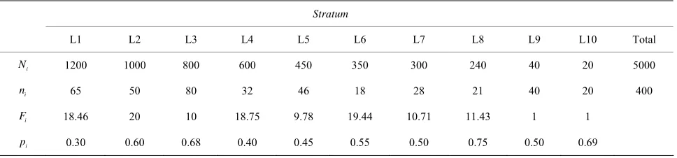
Our first results come from an experiment with binary response. The specific parameter values used to generate the population and the sample are shown in Table 1.

Table 1 summarizes the main features of the experi- ment. Thus, for instance, stratum L1 is formed by 1200 observations taking two possible values, “0” and “1”, that have been randomly generated from Bernoulli trials

with 1 . Note that all the values i

are around 0.5, but there is a high variability between them. The overall population consists of 5000 observa-

tions and satisfies that and

.

"1"

 

ˆ E

 

 

"

1000 p P

  0.05135

 

M 

rel

Under this population design, samples of size were generated, and hence 1000 estimates

 were obtained with each studied method. In the case of the bootstrap procedures, a set of bootstrap replicates was considered to compute each estimator. The behaviour of each estimation procedure was examined by using the following values:

1000 B

  1 1

ˆ M ˆ_r

r

E M

i)   





(iv) MSE ˆ = Bias_  ˆ _2Var ˆ

ii) Bias ˆ E ˆ  (v) RMSE ˆ  MSE ˆ

   

iii) sd ˆ  Varˆ (vi) Effic ˆ MSE ˆ MSE ˆ_PI

 

ˆ

Effic

The quantity  measures the efficiency of each estimator ˆ with respect to the plug-in estimator,

 

ˆ_PI Effic ˆ 1

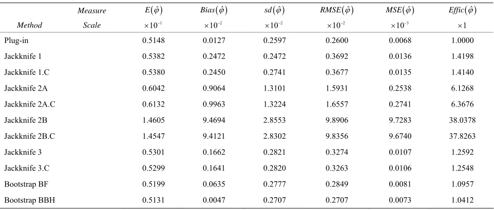
 . Thus,  means that the considered estimator ˆ presents better behavior than the plug-in estimator in terms of mean squared error. Results from our first experiment are shown in Table 2, where different scales have been used to obtain a more intuitive comparison.

Similar experiments were carried out using different

1 L

i i

n n

 



, where the new sample size in the sample sizes 

i-th stratum, i1, , L, was determined by nikni,

with i being the sample size of the first experiment

(see Table 1) and k = 0.25, 0.30, 2, 3 and 4. Excluded from this rule are the two self-represented strata for which obviously

n

i i

n N in all cases. The values of

 

ˆ

RMSE  and Effic

 

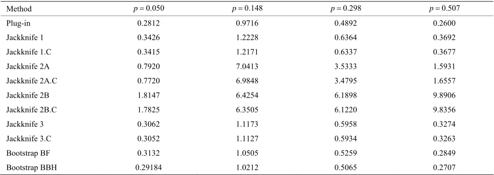
ˆ obtained with these new sample sizes are presented in Tables 3 and 4, respec- tively.

New trials of our first experiment were run with different values of parameter . Table 5 presents

results of

 

"1" pP

 

ˆ

RMSE  obtained for different values of .

p

Tables 2-5 provide a sample of the results obtained in our extensive numerical study with binary response. Some interesting conclusions derived from this study are stated below.

 The plug-in method gave good results and was often the most efficient procedure. Moreover, it has the advantage of being computationally fast. It is also observed that its efficiency improves with increasing sample size.

[image:7.595.57.541.622.735.2]

 

Ni , sample size



n , elevation factor i



Table 1. Parameters in the first experiment with binary response: population size

 

Fi and piP



"1"



for the i-th stratum



Li i



, 1,,10.

Stratum

L1 L2 L3 L4 L5 L6 L7 L8 L9 L10 Total

i

N 1200 1000 800 600 450 350 300 240 40 20 5000

i

n

i

65 50 80 32 46 18 28 21 40 20 400

F 18.46 20 10 18.75 9.78 19.44 10.71 11.43 1 1

i

(8)

[image:8.595.58.539.115.320.2]

Table 2. Results for the experiment with binary response conducted under parameters in Table 1. Total population para- meters: pP



"1"



0 5072. and E_rel



ˆ



0 05135. . Results based on M1000 trials with sample size n400.

Measure E ˆ Bias ˆ sd ˆ RMSE ˆ MSE ˆ Effic ˆ

Method Scale _₁₀1 _₁₀2 _₁₀2 _₁₀2 _₁₀3 _₁

Plug-in 0.5148 0.0127 0.2597 0.2600 0.0068 1.0000

Jackknife 1 0.5382 0.2472 0.2472 0.3692 0.0136 1.4198

Jackknife 1.C 0.5380 0.2450 0.2741 0.3677 0.0135 1.4140

Jackknife 2A 0.6042 0.9064 1.3101 1.5931 0.2538 6.1268

Jackknife 2A.C 0.6132 0.9963 1.3224 1.6557 0.2741 6.3676

Jackknife 2B 1.4605 9.4694 2.8553 9.8906 9.7283 38.0378

Jackknife 2B.C 1.4547 9.4121 2.8302 9.8356 9.6740 37.8263

Jackknife 3 0.5301 0.1662 0.2821 0.3274 0.0107 1.2592

Jackknife 3.C 0.5299 0.1641 0.2820 0.3263 0.0106 1.2548

Bootstrap BF 0.5199 0.0635 0.2777 0.2849 0.0081 1.0957

Bootstrap BBH 0.5131 0.0047 0.2707 0.2707 0.0073 1.0412

 

ˆ 2

10

[image:8.595.57.540.352.522.2]

SE RM

Table 3. Values of   

n n n

for different sample sizes.

Method 145 230 400 740n 1080n n1420

Plug-in 1.1840 0.5366 0.2600 0.127 0.075 0.0052

Jackknife 1 1.5743 0.7060 0.3692 0.298 0.329 0.0380

Jackknife 1.C 1.5737 0.7051 0.3677 0.296 0.325 0.0376

Jackknife 2A 4.3400 2.0697 1.5931 2.572 3.177 0.3616

Jackknife 2A.C 4.2781 2.0474 1.6557 2.660 3.267 0.3707

Jackknife 2B 8.5497 9.0836 9.8906 10.957 11.401 1.1773

Jackknife 2B.C 8.4640 9.0140 9.8356 10.912 11.359 1.1732

Jackknife 3 1.2161 0.6026 0.3274 0.280 0.318 0.0366

Jackknife 3.C 1.2158 0.6021 0.3263 0.277 0.315 40.0362

Bootstrap BF 1.2351 0.5643 0.2849 0.160 0.171 0.0157

Bootstrap BBH 1.2605 0.5715 0.2707 0.137 0.090 0.0072

 

ˆ

Effic

Table 4. Results of  for different sample sizes.

Method n145 n230 n400 n740 n1080 n1420

Plug-in 1.0000 1.0000 1.0000 1.0000 1.0000 1.0000

Jackknife 1 1.3296 1.3156 1.4198 2.3526 4.3525 7.3621

Jackknife 1.C 1.3290 1.3141 1.4140 2.3306 4.3041 7.2785

Jackknife 2A 3.6656 3.8572 6.1268 20.2704 42.0836 70.0182

Jackknife 2A.C 3.6133 3.8156 6.3678 20.9679 43.2797 7107821

Jackknife 2B 7.2211 16.9287 38.0378 86.3640 151.0166 227.9469

Jackknife 2B.C 7.1487 16.7990 37.8263 86.0093 150.4603 227.1530

Jackknife 3 1.0271 1.1230 1.2592 2.2079 4.2156 7.0899

Jackknife 3.C 1.0269 1.1220 1.2548 2.1869 4.1686 7.0090

Bootstrap BF 1.0432 1.0516 1.0957 1.2631 2.2631 3.0474

[image:8.595.56.540.557.734.2]

(9)

 

ˆ 2



10

[image:9.595.56.539.106.278.2]

SE RM

Table 5. Results of    for different values of pP "1"



0.050

p p 0.148

.

Method  0.298p 0.507p

Plug-in 0.2812 0.9716 0.4892 0.2600

Jackknife 1 0.3426 1.2228 0.6364 0.3692

Jackknife 1.C 0.3415 1.2171 0.6337 0.3677

Jackknife 2A 0.7920 7.0413 3.5333 1.5931

Jackknife 2A.C 0.7720 6.9848 3.4795 1.6557

Jackknife 2B 1.8147 6.4254 6.1898 9.8906

Jackknife 2B.C 1.7825 6.3505 6.1220 9.8356

Jackknife 3 0.3062 1.1173 0.5958 0.3274

Jackknife 3.C 0.3052 1.1127 0.5934 0.3263

Bootstrap BF 0.3132 1.0505 0.5259 0.2849

Bootstrap BBH 0.29184 1.0212 0.5065 0.2707

 Both bootstrap methods (BF and BBH) yield competitive results. The BBH bootstrap presents better behaviour than the BF bootstrap, especially for large sample sizes. For moderate or small sample sizes (less than 10% of the population size), the bootstrap methods behave similarly to the plug-in method in terms of efficiency, although with a higher computational cost (that, in any case, results to be acceptable).

 Results in Table 5 allows us to conclude that prior comments are valid for binary variables regardless of the specific value taken by 

 

"1" . In particular, it is observed that RMSE takes the smallest values when p is close to 0 or 0.5.

p P

, ,

Next step in our simulation study is addressed to analyze the case of multiple response. Specifically, it is assumed that there are four mutually exclusive and exhaustive results for the response variable, let us say

1 2 3  The jackknife 3 estimator (based on applying jack-

knife to each stratum) behaved similarly to the boot-

strap estimators for small sample sizes



n400



population of A A A and A4. As in the case of binary response, a and worsened with increasing n. Jackknife 1 esti-

mator (based on leaving out one sample datum) was competitive although yielded worse results than the jackknife 3 with small sample sizes. Both variants of the jackknife 2 estimator (based on leaving out one stratum) yielded much worse results for all the considered sample sizes. Therefore, it is not advisable to use the jackknife 2 estimators. In general, the worse behaviour of the jackknife-based estimators seems to be mainly due to the bias of the estimation, although for the jackknife 2 estimators poor results are also observed in terms of standard deviation.

5000

N observations divided in L = 10 strata was simulated. Data forming the -th stratum were randomly generated from a multinomial distribution with parameter

j



1, 2, ,3 4



j j j j j j

i

    

 , where  de-

notes the probability of event Ai in the -th stratum, j

 

, 1, 2,3, 4

j j

P A i

 i i  . Different values of

j  were selected to set up scenarios with high and low variability of the responses between strata. In all cases, the overall population, which is formed by bringing together all strata, presents the theoretical parameter vector



   1, , ,2 3 4

 

0.58, 0.24, 0.12, 0.06



 

 , where

 

, 1, 2,3, 4

i P Ai i

  

1000 M

.  No substantial differences were observed between

using the jackknife procedures and their corrected versions (.C), based on cancelling the exhaustive strata. Just a slight advantage for the corrected versions is observed.

 Similar conclusions are valid for the two scenarios of high and low variability of the response between different strata. In general, the plug-in estimator is the most efficient in both situations, although the differences between the plug-in and the other methods are smaller in the case of low variability.

 For small sample sizes



n145



, both two bootstrap methods and jackknife 3 led to a greater efficiency than the plug-in method.

A total of  samples of size were randomly selected and each of them was used to con- struct an estimator

400 n

ˆ

 of the relative error in the sam-



1 2 3 4



ˆ ˆ ˆ ˆ ˆ_{, , ,}

pling of      . Again, two strata were considered to be exhaustive in the sampling. The theoretical error for the simulated population is



0.05,0.09,0.15,0.21



 

ˆ ,r1, , M





ˆ ,i1, 2,3, 4



 

ˆ

. The set of estimates obtained with each of the studied methods



r



is

then used to calculate the mean squared error and the efficiency of each procedure with respect to the plug-in method. Both quantities were simultaneously obtained for each estimated marginal component i

(10)

 



 

t ˆ



1 2.

r r



 

 

   1

1

ˆ ˆ M ˆ

r

RMSE MSE

M 



 





   

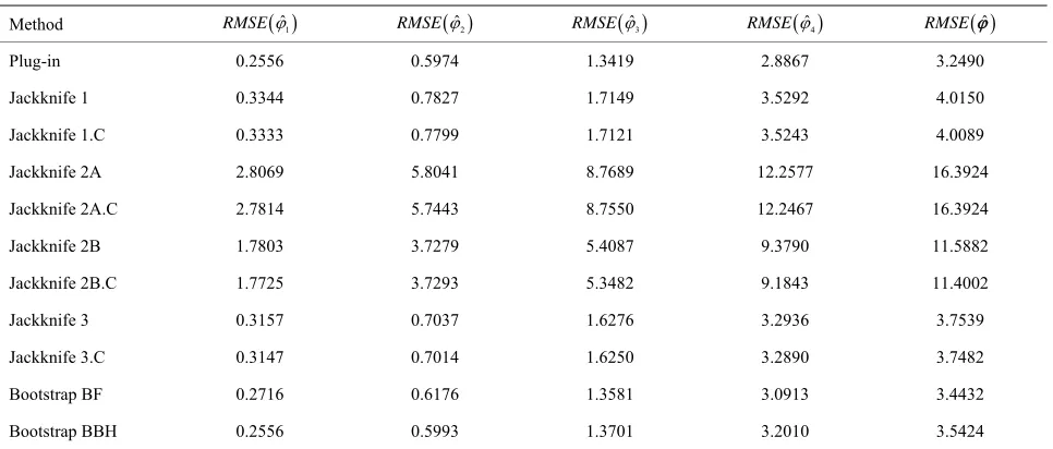
Results from this new simulation are shown in Tables 6 and 7.

Results from Tables 6 and 7 show that the conclusions derived from simulations with binary response are equally valid for the case of multiple response.

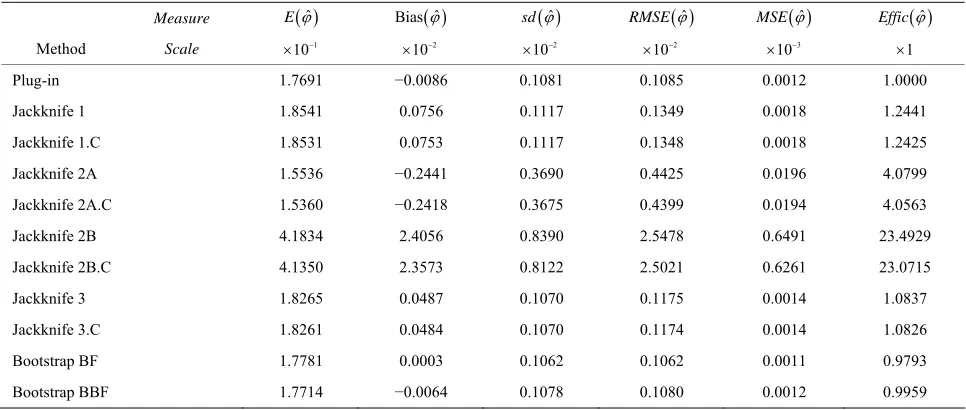
Finally, we focus on the case of continuous response variables. Thus, new experiments were carried out to examine the performance of the different estimation procedures with responses generated from uniform, normal and exponential distributions. The simulation plan was

designed by following the same outline as in previous experiments.

For instance, some experiments with normal and exponential responses were carried out considering the features summarized in Table 8. Note that these parameters lead to a situation of high variability between data from different strata. Some outcomes derived from these experiments are presented in Tables 9 and 10, for the Gaussian case, and in Tables 11 and 12, for the exponential case. Here, the target parameter in the overall population, E_rel

 

ˆ , took the value 0.0177

0.05365

for the Gaussian response, and 



, for the exponential response.

[image:10.595.58.541.285.491.2]



Table 6. Results of ˆ 2

10

RMSE   

1000

M n 400

for the experiment with multiple response and high response variability between strata. Results based on trials with sample size  .

 ˆ1

RMSE RMSE ˆ2 RMSE ˆ3 RMSE ˆ4 RMSE ˆ

Method 

Plug-in 0.2556 0.5974 1.3419 2.8867 3.2490

Jackknife 1 0.3344 0.7827 1.7149 3.5292 4.0150

Jackknife 1.C 0.3333 0.7799 1.7121 3.5243 4.0089

Jackknife 2A 2.8069 5.8041 8.7689 12.2577 16.3924

Jackknife 2A.C 2.7814 5.7443 8.7550 12.2467 16.3924

Jackknife 2B 1.7803 3.7279 5.4087 9.3790 11.5882

Jackknife 2B.C 1.7725 3.7293 5.3482 9.1843 11.4002

Jackknife 3 0.3157 0.7037 1.6276 3.2936 3.7539

Jackknife 3.C 0.3147 0.7014 1.6250 3.2890 3.7482

Bootstrap BF 0.2716 0.6176 1.3581 3.0913 3.4432

Bootstrap BBH 0.2556 0.5993 1.3701 3.2010 3.5424

 

ˆ

[image:10.595.57.540.536.735.2]

Effic

Table 7. Results of  for the experiment with multiple response and high response variability between strata. Results based on M1000 trials with sample size n400

145

n n230 n 400

.

Method  740n 1080n n1420

Plug-in 1.0000 1.0000 1.0000 1.0000 1.0000 1.0000

Jackknife 1 1.1427 1.1322 1.2358 1.6634 2.4630 3.4143

Jackknife 1.C 1.1523 1.1315 1.2339 1.6572 2.4503 3.3943

Jackknife 2A 2.0393 3.2180 5.0454 6.6219 7.4788 7.1866

Jackknife 2A.C 2.0346 3.2084 5.0327 6.6123 7.4769 7.1893

Jackknife 2B 1.5625 2.1351 3.5667 6.5472 10.5012 13.8590

Jackknife 2B.C 1.5410 2.1142 3.5088 6.3559 10.1349 13.3493

Jackknife 3 0.9652 1.0451 1.1554 1.6130 2.3709 3.3767

Jackknife 3.C 0.9818 1.0442 1.1536 1.6071 2.3587 3.3573

Bootstrap BF 1.0101 0.9744 1.0598 1.1614 1.5541 1.8045

(11)

[image:11.595.55.545.122.265.2]

Table 8. Main features for experiments with normal and exponential responses: population size



Ni



, sample size

 

ni

 

Li

and distribution parameters for the i-th stratum .

Stratum

L1 L2 L3 L4 L5 L6 L7 L8 L9 L10 Total

i

N 1200 1000 800 600 450 350 300 240 40 20 5000

i

n

i

65 50 80 32 46 18 28 21 40 20 400

Normal

 50 55 46 45 56 44 57 55 46 50

i

 10 22 15 10 9 20 21 19 11 12

Exponential

i

[image:11.595.56.539.303.508.2]

 0.10 0.11 0.09 0.10 0.11 0.10 0.11 0.09 0.10 0.08

Table 9. Results from the experiment with Gaussian response conducted according to parameters in Table 8 and based on trials with sample size .

= 1000

M n400

Measure E ˆ Bias ˆ sd ˆ RMSE ˆ MSE ˆ Effic ˆ

Method Scale _₁₀1 _₁₀2 _₁₀2 _₁₀2 _₁₀3 _₁

Plug-in 1.7691 −0.0086 0.1081 0.1085 0.0012 1.0000

Jackknife 1 1.8541 0.0756 0.1117 0.1349 0.0018 1.2441

Jackknife 1.C 1.8531 0.0753 0.1117 0.1348 0.0018 1.2425

Jackknife 2A 1.5536 −0.2441 0.3690 0.4425 0.0196 4.0799

Jackknife 2A.C 1.5360 −0.2418 0.3675 0.4399 0.0194 4.0563

Jackknife 2B 4.1834 2.4056 0.8390 2.5478 0.6491 23.4929

Jackknife 2B.C 4.1350 2.3573 0.8122 2.5021 0.6261 23.0715

Jackknife 3 1.8265 0.0487 0.1070 0.1175 0.0014 1.0837

Jackknife 3.C 1.8261 0.0484 0.1070 0.1174 0.0014 1.0826

Bootstrap BF 1.7781 0.0003 0.1062 0.1062 0.0011 0.9793

Bootstrap BBF 1.7714 −0.0064 0.1078 0.1080 0.0012 0.9959

 

ˆ

[image:11.595.60.538.539.733.2]

Effic

Table 10. Results of  for Gaussian response and different sample sizes.

Method n = 145 n = 230 n = 400 n = 740 n = 1080 n = 1420

Plug-in 1.0000 1.0000 1.0000 1.0000 1.0000 1.0000

Jackknife 1 1.2080 1.1241 1.2441 1.9405 3.3611 5.6684

Jackknife 1.C 1.2079 1.2237 1.2425 1.9327 3.3438 5.6372

Jackknife 2A 3.9205 4.5127 4.0799 7.5143 16.6298 31.3715

Jackknife 2A.C 3.9042 4.4950 4.0563 7.5016 16.6140 31.3358

Jackknife 2B 4.4365 10.2989 23.4929 54.3585 93.2693 145.4229

Jackknife 2B.C 4.3642 10.1115 23.0715 53.5200 91.8624 143.3255

Jackknife 3 0.9942 1.0336 1.0837 1.8723 3.2635 5.5708

Jackknife 3.C 0.9943 1.0335 1.0826 1.8648 3.2468 5.5406

Bootstrap BF 1.0140 0.9996 0.9793 1.0183 1.8710 2.0230

(12)

[image:12.595.57.539.110.297.2]

Table 11. Results from the experiment with Exponential response conducted according to parameters in Table 8 and based on M = 1000 trials with sample size n = 400.

Measure E ˆ Bias ˆ sd ˆ RMSE ˆ MSE ˆ Effic ˆ

Method Scale _₁₀1 _₁₀2 _₁₀2 _₁₀2 _₁₀3 _₁

Plug-in 5.3474 −0.0179 0.2894 0.2899 0.08410 1.0000

Jackknife 1 5.5928 0.2275 0.2915 0.3698 0.1368 1.2756

Jackknife 1.C 5.5928 0.2252 0.2917 0.3685 0.1358 1.2710

Jackknife 2A 2.4534 −2.9119 0.8971 3.0470 9.2841 10.5098

Jackknife 2A.C 2.4865 −2.8788 0.9022 3.0168 9.1013 10.40556

Jackknife 2B 6.4268 1.0615 2.1040 2.3566 5.5537 8.1284

Jackknife 2B.C 6.3898 1.0245 2.0803 2.3402 5.4766 8.0719

Jackknife 3 5.5246 0.1593 0.3012 0.3407 0.1161 1.1751

Jackknife 3.C 5.5224 0.1571 0.3013 0.3398 0.1154 1.1719

Bootstrap BF 5.3963 0.0310 0.2991 0.3007 0.0904 1.0371

Bootstrap BBH 5.3442 −0.0211 0.2921 0.2928 0.0857 1.0100

 

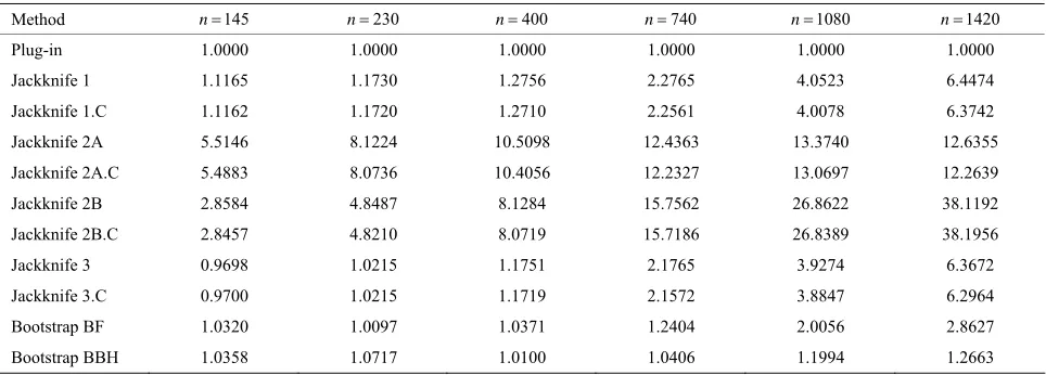
ˆ

[image:12.595.57.539.329.502.2]

Effic

Table 12. Results of  for exponential response and different sample sizes.

Method n145 230n 400n 740n 1080n n1420

Plug-in 1.0000 1.0000 1.0000 1.0000 1.0000 1.0000

Jackknife 1 1.1165 1.1730 1.2756 2.2765 4.0523 6.4474

Jackknife 1.C 1.1162 1.1720 1.2710 2.2561 4.0078 6.3742

Jackknife 2A 5.5146 8.1224 10.5098 12.4363 13.3740 12.6355

Jackknife 2A.C 5.4883 8.0736 10.4056 12.2327 13.0697 12.2639

Jackknife 2B 2.8584 4.8487 8.1284 15.7562 26.8622 38.1192

Jackknife 2B.C 2.8457 4.8210 8.0719 15.7186 26.8389 38.1956

Jackknife 3 0.9698 1.0215 1.1751 2.1765 3.9274 6.3672

Jackknife 3.C 0.9700 1.0215 1.1719 2.1572 3.8847 6.2964

Bootstrap BF 1.0320 1.0097 1.0371 1.2404 2.0056 2.8627

Bootstrap BBH 1.0358 1.0717 1.0100 1.0406 1.1994 1.2663

Results in Tables 9-12 allow us to confirm that the different analyzed estimation procedures behaved as in the previous experiments. Moreover, an analogous behaviour was also observed with uniform response and with scenarios of low variability between strata. In short, the conclusions derived from our numerical study with binary or multinomial response can be extended to the case of continuous response variables, regardless of the gene- rating probability distribution.

amined in this type of surveys are binary, categorical and continuous, and hence, the estimates of interest involve estimates of proportions, totals and means. In this setting, several procedures to approximate the sampling relative error of this kind of estimates are proposed. Different estimation techniques are considered, including the natu- ral estimation of plug-in type and more sophisticated methods based on jackknife and bootstrap methodologies. The behaviour of the different procedures proposed is examined and compared by means of an extensive simulation study. In general, the plug-in method presents good behaviour in all the analyzed situations, with the additional advantage of having a low computational cost. For small sample sizes, the jackknife estimator denoted by “jackknife 3”, which is based on the prior application of the jackknife technique to each stratum, and the two bootstrap methods considered (particularly the bootstrap proposed by Booth, Butler and Hall) yield results similar

6. Final Conclusion

(13)

as those obtained with the plug-in estimator, and in some cases, even better. However, the estimators obtained with these methods have a higher (although acceptable) computational cost.

7. Acknowledgements

This research was supported by the Galician Official Statistical Institute (IGE) and by Grants 10DPI105003PR and CN2012/130 from Xunta de Galicia (Spain), and by Grant number MTM2011-22392 from Ministerio de Ciencia e Innovación (Spain).

REFERENCES

[1] S. K. Thompson, “Sampling,” Wiley, New York, 1992. [2] M. Quenouille, “Approximate Tests of Correlation in

Time Series,” Journal of the Royal Statistical Society: Se- ries B (Statistical Methodology), Vol. 11, No. 1, 1949, pp.

18-84.

[3] B. Efron, “Bootstrap Methods: Another Look at the Jackknife,” The Annals of Statistics, Vol. 7, No. 1, 1979,

pp. 1-26. doi:10.1214/aos/1176344552

[4] B. Efron, “The Jackknife, the Bootstrap, and Other Re- sampling Plans, Siam Monograph 38,” Society of Indus- trial and Applied Mathematics CBMS-NSF Monographs, 1982.

[5] B. Efron and R. Tibshirani, “An Introduction to the Boot- strap,” Chapman & Hall, New York, 1993.

[6] P. J. Bickel and D. A. Freedman, “Asymptotic Normality and the Bootstrap in Stratified Sampling,” The Annals of Statistics, Vol. 12, No. 2, 1984, pp. 470-482.

doi:10.1214/aos/1176346500

[7] J. G. Booth, R. W. Butler and P. Hall, “Bootstrap Meth- ods for Finite Populations,” Journal of the American Sta- tistical Association, Vol. 89, No. 248, 1994, pp. 1282-