An Approximation Method for a Maximum Likelihood Equation System and Application to the Analysis of Accidents Data

http://www.scirp.org/journal/ojs ISSN Online: 2161-7198

ISSN Print: 2161-718X

An Approximation Method for a Maximum

Likelihood Equation System and Application to

the Analysis of Accidents Data

Assi N’Guessan

1

, Issa Cherif Geraldo

2

, Bezza Hafidi

3

1_{Laboratoire Paul Painlevé (UMR CNRS 8524), Université de Lille 1, Villeneuve d’Ascq, France}

2_{Department of Mathematics and Computer science, Université Catholique de l’Afrique de l’Ouest-Unité Universitaire du Togo,} Lomé, Togo

3_{Department of Mathematics, Faculty of Science, University Ibn Zohr, Agadir, Morocco}

Abstract

There exist many iterative methods for computing the maximum likelihood estimator but most of them suffer from one or several drawbacks such as the need to inverse a Hessian matrix and the need to find good initial approxima-tions of the parameters that are unknown in practice. In this paper, we present an estimation method without matrix inversion based on a linear approxima-tion of the likelihood equaapproxima-tions in a neighborhood of the constrained maxi-mum likelihood estimator. We obtain closed-form approximations of solu-tions and standard errors. Then, we propose an iterative algorithm which cycles through the components of the vector parameter and updates one component at a time. The initial solution, which is necessary to start the itera-tive procedure, is automated. The proposed algorithm is compared to some of the best iterative optimization algorithms available on R and MATLAB soft-ware through a simulation study and applied to the statistical analysis of a road safety measure.

Keywords

Constrained Maximum Likelihood, Partial Linear Approximation, Schur’s Complement, Iterative Algorithms, Road Safety Measure, Multinomial Model

1. Introduction

Approximation methods for Maximum Likelihood (ML) systems of equations are of interest and are motivated in this paper by the need to find estimation methods that are simple and easy to implement in the specific field of the

How to cite this paper: N’Guessan, A., Geraldo, I.C. and Hafidi, B. (2017) An Approximation Method for a Maximum Likelihood Equation System and Applica-tion to the Analysis of Accidents Data. Open Journal of Statistics, 7, 132-152.

http://dx.doi.org/10.4236/ojs.2017.71011

Received: August 8, 2016 Accepted: February 25, 2017 Published: February 28, 2017

Copyright © 2017 by authors and Scientific Research Publishing Inc. This work is licensed under the Creative Commons Attribution International License (CC BY 4.0).

http://creativecommons.org/licenses/by/4.0/

statistical evaluation of the impact of a road safety measure. In practice, the estimation methods dedicated to this evaluation depend both on the nature of the measure and the available data. Methods based on frequencies combination have received considerable attention [1] [2][3] and for the most part of them, we are faced with the estimation of unknown parameters which are often functionally dependent.

Many approximation methods for maximum likelihood estimation need to solve systems of linear or non-linear equations with or without constraints

[4]-[9]. Newton-Raphson’s method and Fisher scoring are certainly the most

commonly used approximation methods. They consist in updating the whole parameter vector using the iterative scheme:

( ) ( )

( )

( ) 1

( )

( )

1

k k k k

M

φ + ₌φ ₊ φ − _∇ φ

   (1) where φ( )k _{is the estimate of the vector parameter at the step}

k,  is the log-likelihood function,

( )

_φ( )k

∇ is the gradient of  and

( )

( )k

M φ is the observed or the expected information matrix. Both methods require the com- putation of second-order partial derivatives and a matrix inversion in each iteration, which can be very costly. Some authors such as Wang [10] have proposed quadratic approximations and extended Fisher scoring. The main point is to use quadratic approximations to the log-likelihood function and optimize these approximations within the constrained parameter space.

Within the framework of crash data analysis, different iterative estimation methods have been proposed [2][11]. For example, Mkhadri et al. [11] propose a Minorization-Maximization (MM) algorithm for the maximum likelihood estimation of the parameter vector of a multinomial distribution modelling crash data. Their proposed MM algorithm cycles through the components of the parameter vector and updates one component at a time which leads to closed-form expressions of the parameters. They claim that their MM algorithm is simple to implement without any matrix inversion and constraints are integrated easily.

Despite the above advantages, the choice of the starting value _φ( )0

remains a major issue since a value of φ( )0 _{relatively far from the true unknown value of}

the vector parameter can lead to erroneous solutions or to non-convergence. In addition to this, it must be noted that obtaining explicit expressions of standard errors is not generally easy.

The remainder of the paper is organized as follows. Section 2 is devoted to the statistical model and the main assumptions used to get closed-form appro- ximations and standard errors. The proposed estimation method and the method for computing standard errors are presented in Section 3. The general framework of the proposed algorithm is also described. In Section 4, we give an illustration of our results using a crash data model. The numerical performance of the proposed algorithm is examined in Section 5 through a simulation study while a real-data application is given in Section 6. The appendix is devoted to the technical details of the main results.

2. Statistical Model and Main Assumptions

2.1. Statistical Model

Let Y =

(

Y11,,Y Y1r, 21,,Y2r

)

be a random vector with 2r r

(

>1

)

compo-

nents and π φ

( )

=

(

π φ11

( )

,,π φ π φ1r

( )

, 21

( )

,,π φ2r

( )

)

be a vector of pro-

babilities such that

( )

2 1 1

1

r ij i j

π φ

= =

=

∑∑

where

φ

is a parameter vector. It is assumed that the vector Y has the multinomial distribution 

(

n;π φ

( )

)

where n>0 is a known integer. The basic principle of the multinomial distribution 

(

n;π φ

( )

)

consists in dis-

tributing n items in 2r categories or classes (2r being the number of com- ponents of vector π φ

( )

_{). The probability for an object to fall in a class is called} class probability with the sum of all class probabilities equal to 1. Here, the class probabilities π φij

( )

depend on the unknown vector parameter

φ

.

Given a vector of integers y=

(

y11,,y1r,y21,,y2r

)

such that

2 1 1

,

r ij i j

y n

= =

=

∑∑

the probability function related to 

(

n;π φ

( )

)

is defined by

( )

2

(

( )

)

2

1 1

1 1

!

. !

ij

r _y

ij r

i j ij i j

n f y

y = = π φ

= =

=

∏∏

∏ ∏

(2)

2.2. ML Estimation and Main Assumptions

Assumption 1. The vector parameter

φ

_{is partitioned as} φ=

(

θ β,

)

where

0

θ

> _{is a real parameter,}

₍

₎

T 1, , r

β = β  β is a vector and

β

j >0 for all 1, ,

j=  r.

Assumption 2. The unknown vector

φ

is subject to a linear constraint

( )

0

C φ = where C is a continuously differentiable function from r+1 to

.

Let

(

)

2

11, , 1 , 21, , 2

r

r r

( )

( )

Maximize  φ subjet to C φ =0. (3)

Problem (3) is equivalent to the maximization of function

(

φ λ,

)

=

( )

φ −λ φC

( )

 (4) where

λ

_{is the Lagrange multiplier. The information matrix linked to the}

constrained maximum likelihood estimator _φˆ _is

T T

, 0

J C U

J

C U B

φ φ φ φ

φ φ

φ φ φ

τ

   

Γ =  = 

   

    (5)

where

(

)

T ₁

1

, , , r

r

C_φ = ∂ ∂ ∂ ∂C θ C β  ∂ ∂C β ∈+ , Jφ∈1+r×1+r,

2 2 2

2

1

, , ,

r

E U E

φ φ

τ

θ β θ β

θ  ∂   ∂ ∂  = _− _∈ = _− − _ ∂ ∂ ∂ ∂ ∂      _  _ 

and Bφ is a r×r matrix whose entries are E

(

−∂2 ∂ ∂β βm j

)

, m j, =1,,r.

We also assume that the following conditions are verified:

Assumption 3. ∂ ∂ =C θ 0 and C_β,β = ≠κ 0 where .,. is the inner

product, κ is a constant and

(

)

T 1, ,

r r

C_β = ∂ ∂C β  ∂ ∂C β ∈ ;

Assumption 4. For any

θ

>0, there exists a non-singular r×r matrix

ˆ,y θ

Ω _{such that} T 1 ˆ ˆ,y ˆ 0

C_βΩ_θ− C_β > and the non-linear system

ˆ ˆ

ˆ _ˆ

ˆ,

0

ˆ, C r

C φ β φ _β β β β _β ∂  _∂    ∂  _{− =} _∂     

is approximated by the linear system

ˆ, ˆ

T ˆ

ˆ

0 0

y C D_y

C θ β β β κ Ω  _{    } =  _{    }       

where

(

)

T

0_r = 0,, 0 ∈r and D_y is a r×1 vector whose components are obtained from y.

Assumption 5. There exists a function 1

: r

g − → such that the equation

ˆ 0 φ θ ∂  _{ =} _∂   

 _{is equivalent to ˆ}

_{( )}

_ˆ

g

θ = β _.

Assumption 6. There exist two strictly positive real numbers an,φ and bn,φ,

a non-singular r×r diagonal matrix Σ_φ and a vector Vφ∈r such that 1 2

, ,

n n

a b

φ φ φ

τ ₌ − _,

(

T

)

,

n

B_φ =a _φ Σ +_φ V V_{φ φ} and U_φ =b V_{n,φ φ}.

Assumption 3 specifies the form of function C. Particularly, C is only a function of sub-vector

β

. Assumptions 4 and 5 enable us to get _βˆ _{from θ}ˆ and inversely. Assumption 6 enables us to transform the Fisher information matrix in order to use classical results on matrix inversion with Schur’s com- plement [17].

3. The Estimation Method

3.1. Partial Linear Approximation Principle

has been discussed by many authors [12] [13] [14]. The classical approach is based on a Newton-type algorithm and computes the components of _φˆ _{at once.}

Except from some few simple cases, it is not generally possible to get explicit expressions of the components of _φˆ_{. One shows the following lemma (we refer}

the reader to the appendix for a proof).

Lemma 1. The constrained maximum likelihood estimator _φˆ_{, provided it}

exists, is solution to the non-linear system

ˆ ˆ

ˆ ˆ _ˆ

ˆ,

0 and 0

ˆ, C r

C

φ β

φ φ _β

β β

θ β _β

∂  _∂ 

 

 

∂ ∂

 _{ = − =}

_∂  _∂ 

   



  ₍₆₎

where

(

)

T

0r = 0,, 0 ∈r.

Our approach consists in dividing Equation (6) into two parts: one con- cerning the first component of _φˆ _{and the other one concerning the sub-vector}

ˆ

β.

Theorem 1. Under assumptions 3 - 5, the constrained MLE _φˆ₌

( )

_{θ β}ˆ ˆ_{, is} given by:

( )

ˆ _g ˆ

θ= β

1 ˆ,

ˆ _.

y yD

θ

β _{= Ω}−

The non-obvious part of the proof consists in the determination of _βˆ _by

inverting the

(

r+ × +1

) (

r 1

)

matrix linked to the linear system in Assumption

4. This result based on the inversion of partitioned matrices will not be demonstrated in this paper. We refer the reader to classical papers on Schur complement [15][16].

From Theorem 1, it is seen that the MLE _φˆ₌

( )

_{θ β}ˆ ˆ_{, is a fixed point of the} function from _r+1 _{to itself defined by}

(

)

(

( )

1

)

,

, g , _θyD_y

θ β _ β _Ω− _{. We can then}

build an iterative algorithm to estimate

φ

_{. The classical fixed point method}

which consists in simultaneously updating _θˆ _{and β}ˆ _{may be hard to im-}

plement because of the link between _θˆ _{and β}ˆ_{. We propose instead to alternate}

between updating _θˆ _{holding β}ˆ _{fixed and vice-versa. Starting from a given} ( )0

θ

, we compute _β( )0 _{and then}

θ

( )1 _{and β}( )1 _{and so on. The process is}

repeated until a stopping criteria is satisfied. For example, we can stop the iterations when successive values of the log-likelihood satisfy the condition

( )

( )

_φk+1 ₋

( )

_φ( )k _<

   where >0.

The estimation process may be completed by the computation of standard errors with Theorem 2 below.

Theorem 2. Under assumptions 3 - 6, the asymptotic variance of the com- ponents of _φˆ _are

( )

1 1

ˆ ˆ

2 2

2 2 2

ˆ ˆ ˆ ˆ ˆ

, ,

ˆ

ˆ a_n b_n 1 V C

φ φ

φ φ φ β φ

σ θ − ₋ −₋ ξ

Σ Σ

 

= _ + − _

  (7)

( )

1

(

)

ˆ

2 2

2 1 1 1

ˆ ˆ ˆ ˆ ˆ

, , , ,

ˆ

ˆ j an j C j C j , j 1, ,r

β

φ φ β φ β

σ β − − −₋ −

Σ

 

= _Σ − × Σ × _ =

   (8)

where T 1

0

V C

φ φ φ β

ξ _{= Σ}− _{> and the real values} 1 ,j φ−

Σ (resp. Cβ,j), j=1,,r,

are the diagonal elements (resp. components) of matrix 1 φ−

Σ (resp. of vector C_β).

The proof is given in the appendix. It stems from the results of N'Guessan and Langrand [17].

3.2. General Framework of the Partial Linear

Approximation Algorithm

Algorithm 1 (The partial linear approximation algorithm). Step 0 (Initialization) Given

_θ

( )0

, >0, D_y, compute ( ) ( )0

0 1

,yDy

θ

β _{= Ω}− _.

Step 1 (Loop for computing _φˆ_{)For a given k≥0,}

a) Compute ( )k1

( )

( )k

g

θ + ₌ β

and ( )

( 1)

1 1

, k

k

y yD

θ

β +

+ _{= Ω}− _.

b) If _

( )

_φ( )k+1 _−

( )

_φ( )k _≥

, then replace k by k+1 and return to Step 1. Else, set

_{θ θ}

_ˆ= ( )k+1 _, β β_ˆ= ( )k+1

and go to Step 2. Step 2 (Computation of standard errors)

a) Compute

( )

1 1

ˆ ˆ

2 2

2 2 2

ˆ ˆ ˆ ˆ ˆ

, ,

ˆ

ˆ a b_{n n} 1 V C

φ φ

φ φ φ β φ

σ θ − ₋ −₋ ξ

Σ Σ

 

= _ + − _

 .

b) For j=1,,r, compute

( )

(

)

1

ˆ

2 2

2 1 1 1

ˆ ˆ ˆ ˆ ˆ

, , , ,

ˆ ˆ _j

n j j j

a C C

β

φ φ β φ β

σ β − − −₋ −

Σ

 

= _Σ − × Σ × _

 .

The aim of this paper is not to conduct a theoretical study of the convergence of the proposed algorithm. We rather focus on the numerical aspect of this convergence through an application model. Nevertheless, we can notice that the estimation of _φˆ _{using our algorithm does not require any matrix inversion. It}

is thus easy to think that getting the constrained maximum likelihood estimator

ˆ

φ _{is improved in terms of computation time.}

4. Application to the Combination of Crash Data

4.1. Statistical Model

We apply the above algorithm to estimate the parameters of a statistical model used to assess the effect of a road safety measure applied to an experimental site presenting r>0 mutually exclusive accident types (fatal accidents, seriously injured people, slightly injured people, material damage, etc) over a fixed period. Let us consider the random vector Y =

(

Y11,,Y Y1r, 21,,Y2r

)

where

1j

Y and Y_2j

(

j=1,,r

)

respectively represent the number of accidents of type

j registered on the experimental site before and after the application of the road safety measure. In order to take into account some external factors (such as traffic flow, speed limit variation, weather conditions, regression to the mean effect, etc), the experimental site is linked to a control area where the safety measure was not directly applied. The accidents data for the control area over the same period is given by the non-random vector

(

)

T

1, , r

after to the number of accidents of type j registered in the period before. Following N’Guessan et al. [18], we assume that the vector Y has the multi- nomial distribution

( )

(

,

)

Y ∼M nπ φ

where n is the total number of crashes recorded at the experimental site and

(

11, , 1r, 21, , 2r

)

π = π π π π is a vector of class probabilities whose components are

( )

1

1

1

if 1; 1, ,

1

if 2; 1, , .

1 j r m m m ij r

j m m m r

m m m

i j r

z

z

i j r

z β θ β π φ θβ β θ β = = =  = =  +  =   _{= =}  + 

∑

∑

∑

  (9)

By construction, the parameter vector φ=

(

θ β,

)

of this model satisfies the

conditions

θ

>0,

β

j >0 and the linear constraint

( )

0, with

( )

1 ,_r 1

C φ = C φ = β − (10) where 1r=

(

1,,1

)

∈r. The scalar

θ

denotes the unknown parameter average effect of the road safety measure while each β_j

(

j=1,,r

)

denotes the risk of having an accident of type j on a site having the same characteristics as the experimental site. This model is a special case of the multinomial model proposed by N’Guessan et al. [18] which was applied simultaneously on several sites.

4.2. Cyclic Estimation of the Average Effect and the

Different Accident Risks

The log-likelihood is specified up to an additive constant by

( )

.

( )

2

( )

. 2

1 1 1

log log log 1 log

r r r

m m m m j j m j j

m j j

y y y z y z

φ β θ θ β β

= = =      = _ + − _ + _+ _{ }       

∑

∑

∑

 (11)

where y.m=y1m+y2m. Different iterative methods can be used to compute the

constrained MLE _φˆ_{. Most of them look for stationary points of the Lagrangian}

(

) ( )

1

, 1 .

r m m

φ λ φ λ β

=   = − _ − _ 

∑

  

N'Guessan et al. [18] showed that a stationary point of 

(

φ λ,

)

must be the

solution to the following system of non-linear equations:

( )

( )

(

)

( )

( )

(

)

( )

2 . 1 2. . ˆ ˆ 0 ˆ ˆ 1

ˆ ₁ ˆ ˆ ˆ

0, 1, ,

ˆˆ ˆ

1

ˆ _{0, 0, 1,}ˆ _,

r

m m m

j j j j

j

j

E Z

y y

E Z

n z y E Z z

y j r

E Z E Z

j r

θ θ

β θ β

θ θ β =    − =  _ _ +     +  −  _{− − = =}  + 

where 2. 1 2

r m m

y =

∑

₌y and

( )

1

ˆ

ˆ r

m m m

E Z =

∑

₌β z .

The main idea proposed in this paper consists in neglecting the term

( )

(

)

( )

2.ˆj ˆ j ˆ

y β E Z z E Z

 ₋ 

  so that we can write the remaining equations

(

)

( )

.

ˆ ₁ ˆ

0, 1, ,

ˆ ˆ 1

j j

j

n z

y j r

E Z β θ θ + − = = + 

as the linear system of equations

ˆ,yˆ Dy

θ β

Ω = (13)

where T

ˆ_,y Mˆ ˆD Zy

θ θ θ

Ω = − , M_θˆ =diag 1

(

+θˆz1,,1+θˆzr

)

is a diagonal r×r

matrix and

T

11 21 1 2

, , r r r.

y

y y y y

D n n + +   =_{ } ∈    

Drawing our inspiration from the work by N'Guessan [19], we show that the linear system (13) has the vector

(

T 1

)

1 1

ˆ ˆ

ˆ ₁ ˆ

y y

Z M D_θ M D_θ

β _{= −}θ − − − _{as unique so-}

lution. One shows that

(

T 1

)

ˆ

1

ˆ 1 ˆ

1 1 .

ˆ 1 r m m y m m z y Z M D

n z θ θ θ θ − ⋅ = − = − +

∑

The components of the constrained MLE _φˆ _{can then be computed as}

follows.

Corollary 1. The components of _φˆ₌

( )

_{θ β}ˆ ˆ_{, are given by}

(

) (

1 2

)

1 1 1 ˆ ˆ r m m r r

m m m

m m y z y

θ

β

= = = = ×

∑

∑

∑

(14)

( )

.

1 1

ˆ _{, 1, ,}

ˆ ˆ ₁ 1 j j j n y j r n z β θ θ = × × = +

− ∆  (15)

where

( )

1 ˆ 1 ˆ ˆ 1 r m m n m _m z y n z θ θ θ ⋅ = ∆ = +

∑

.

Applying Theorem 2’s results, we can give the asymptotic variance of the constrained MLE _φˆ_.

Corollary 2. The asymptotic variance of the components of the constrained maximum likelihood estimator _φˆ _{is given by}

( )

_{( )}

( )

( )

(

)

( )

2

2 2 3

2 ˆ ˆ 1 1 ˆ ˆ ˆ 1 ˆ _ˆ

E Z E Z

n n

nE Z _{E Z}

σ θ θ θ θ

    = + _ + _ +     (16)

( )

(

)

2 _ˆ 1 _{ˆ ˆ}

ˆ _{j j} 1 _j , j 1, ,r

n

σ β = β −β =  (17)

where

( )

1

ˆ

ˆ r

m m m

E Z =

∑

₌β z and

( )

2 2 1

ˆ

ˆ r

m m m

E Z =

∑

₌β z .

(

)

T 1 2

( )

2

(

T

)

0,1, ,1 r, E Z , ,

C U Z B V V

n n

φ φ φ φ φ φ φ

γ

γ

τ

γ

θ

+

=  ∈ = = = Σ + (18)

where

( )

( )

1 2

1

1 1

, diag , , , .

1

r

n n

V Z

nE Z E Z

φ φ

θγ _γ

γ β β θ

   

=_ _ Σ = ×   = ₊

 

   (19)

Setting an,φ =

γ

and

(

( )

)

( )

2 3

,

n

b _φ = γ E Z nθ , we show that Assumption 6 is satisfied. We then apply Theorem 2 to get the results of Corollary 2.

4.3. Practical Aspect of the Partial Linear Approximation

Algorithm

Algorithm 2.

Step 0 (Initialization) Given >0 and D_y, set

θ

( )0 =0 and compute

( )0

y

D β = _.

Step 1 (Loop for computing _φˆ_{) For a given k≥0,}

a) Compute ( ) _{( )}

(

) (

)

1 1 2

1

1 1

r

k m m

r k r

m m m

m m y z y

θ

β

+ = = = = ×

∑

∑

∑

b) For j=1,,r, compute

( ) ( ) ( ) ( ) . 1 1 1 . 1 1 1 1 . 1 1 1 1 j k

j _r k k

m m j

k

m _m

y

n

z y z

n z β θ θ θ + + + + = = × × + − +

∑

c) If _

( )

_φ( )k+1 _−

( )

_φ( )k _≥

, then replace k by k+1 and return to Step 1. Else, set

_{θ θ}

_ˆ= ( )k+1

, β β_ˆ= ( )k+1 and go to _{Step 2.}

Step 2 (Computation of standard errors)

a) Compute

( )

_{( )}

( )

( )

(

)

( )

2

2 2 3

2 ˆ ˆ 1 1 ˆ ˆ ˆ 1 ˆ _ˆ

E Z E Z

n n

nE Z _{E Z}

σ θ θ θ θ

    = + _ + _ +     .

b) For j=1,,r, compute _ˆ2

( )

_ˆ 1 _ˆ

(

_ˆ

)

1

j j j

n

σ β = β −β _.

The partial linear approximation algorithm for computing the constrained maximum likelihood estimator _φˆ _{of the model presented in subsection 4.1}

stems from the cyclic algorithm of N’Guessan and Geraldo [20]. The PLA proceeds as follows: step 1 allows to estimate _φˆ _{alternating between its two}

components _θˆ _{et β}ˆ_{. To start the procedure, we initialize}

_θ

( )0

. Then we compute ( )0

(

)

1, ,

j j r

β =  and define ( )0

(

( )0 ( )0

)

,

φ = θ β . But, we could also initialize _β( )0

using the problem’s data and get

θ

( )0

. The process is repeated until the stopping criterion is satisfied. We note that our algorithm is automated and can be started as soon as the problem’s data Dy is entered.

5. Numerical Results with Simulated Datasets

5.1. Data Simulation Principle

For a given value of r (the number of crash types), we generate the com- ponents of vector

(

)

T

1, , r

Z = z  z from a uniform random variable 1 5, 2 2 U_ _

 . The true value of

θ

denoted θ0 is fixed and the true value of

β

, denoted

(

)

T

0 0 0

1, , r

β = β  β , such that 0

1 1

r j j=β =

∑

, comes from a uniform random variable U

(

,1−

)

where 5

10− =

 . Using those values, we compute the true probabilities

( )

0

( )

0 0 0

0 0 1

1 _{0 0} 2 _{0 0}

1 1

, , 1, ,

1 1

r

j j m m m

j r j r

m m m m

m m

z

j r

z z

β θ β β

π φ π φ

θ β θ β

=

= =

= = =

+ +

∑

∑

∑



linked to the multinomial distribution presented in subsection 4.1. Finally, one generates the total number n of crash data from a Poisson distribution and then randomly shares it between the before and after periods using probabilities

( )

0 1j

π φ and

( )

0 2j

π φ . The observed values of yij such that

2 1 1

r ij i= j=y =n

∑ ∑

are then found.

5.2. Numerical Results

This subsection deals with the numerical convergence of the partial linear approximation algorithm. As usual in the study of iterative algorithms, we analyse the influence of the initial solution ( )0

(

( )0 ( )0

)

,

φ = θ β , the number of iterations, the computation time (CPU time) and the mean squared error. The performances of the partial linear approximation algorithm are compared to those of some classical optimization methods available in R and MATLAB software. The computations presented in this section were executed on a PC with an AMD E-350 Processor 1.6 GHz CPU.

The methods selected for comparison are the Newton-Raphson’s method, Nelder-Mead’s (NM) simplex algorithm [21], quasi-Newton BFGS algorithm (from the names of its authors Broyden, Fletcher, Goldfarb and Shanno [22][23] [24] [25]), Interior Point (IP) algorithm [26], the Lenverberg-Marquardt (LM) algorithm [27] [28] and Trust Region (TR) algorithms [29]. In our work, the BFGS and NM algorithms are implemented using the package developed by Varadhan [30].

The simulation process was performed on many simulated crash datasets. For each one, small and large values of n were considered. The results presented here correspond to the case r=3, n∈

{

50;5000

}

, φ0=

(

θ β0, 0

)

with θ =0 0.6

and 0

(

)

0.025, 0.232, 0.743

β = .

Three different ways of setting _β( )0

were considered: 1) Uniform initialisation: ( )0 ( )0 ( )0

1 2 r 1r

β =β ==β = .

2) Proportional initialisation: ( )0 1j 2j j

y y

n

β = + , j=1,,r.

(

1, ,

)

i

u i=  r is randomly generated from an uniform distribution

(

0.05, 0.95

)

U .

By combining the two values of n and the three ways to initialize β( )0 , we get six scenarios and for each one, we performed 1000 replications. The stopping criterion is the condition

( )

( )1

( )

( ) 5

10

k k

φ + ₋ φ _< −

  .

Tables 1-6 present a few of the results obtained for an overall 6000 simu-

[image:11.595.204.539.202.452.2]

lations. All computation times are given in seconds and the duration ratio of an

Table 1. Results for uniform initialisation of β( )0 _,

3

r= , n=50.

R software MATLAB software

PLA NR BFGS NM PLA LM TR IP

ˆ

φ 0.621 0.617 0.617 0.618 0.643 0.639 0.639 0.639

0.060 0.054 0.054 0.054 0.060 0.054 0.054 0.054 0.207 0.227 0.227 0.227 0.203 0.223 0.223 0.223 0.733 0.719 0.719 0.719 0.737 0.723 0.723 0.723 Min.

iterations 2 2 11 8 2 3 2 8

Max.

iterations 4 4 11 19 4 4 11 22

Mean

iterations 3.1 3.0 11.0 12.1 3.1 3.2 5.8 13.8

CPU time 7.64E−04 3.84E−03 1.83E−01 2.85E−01 1.41E−03 4.37E−02 5.07E−02 4.97E−01 Duration

ratio 1 5 239 373 1 31 36 353

[image:11.595.204.539.480.728.2]

MSE 9.90E−03 9.74E−03 9.74E−03 9.79E−03 1.12E−02 1.09E−02 1.09E−02 1.09E−02

Table 2. Results for uniform initialisation of β( )0 _,

3

r= , n=5000.

R software MATLAB software

PLA NR BFGS NM PLA LM TR IP

ˆ

φ 0.604 0.601 0.601 0.602 0.604 0.601 0.601 0.601

0.028 0.025 0.025 0.025 0.028 0.025 0.025 0.025 0.212 0.232 0.232 0.233 0.212 0.232 0.232 0.232 0.760 0.743 0.743 0.742 0.760 0.743 0.743 0.743 Min.

iterations 4 3 15 12 4 3 3 9

Max.

iterations 4 4 15 20 4 4 12 21

Mean

iterations 4.0 3.3 15.0 15.1 4.0 3.0 6.4 13.7

CPU time 9.35E−04 4.11E−03 3.23E−01 3.54E−01 1.71E−03 4.24E−02 5.30E−02 5.33E−01 Duration

ratio 1 4 345 379 1 25 31 311

[image:12.595.208.538.91.333.2]

Table 3. Results for proportional initialisation of _β( )0 _,

3

r= , n=50.

R software MATLAB software

PLA NR BFGS NM PLA LM TR IP

ˆ

φ 0.626 0.622 0.622 0.623 0.632 0.628 0.628 0.628

0.061 0.055 0.055 0.055 0.060 0.053 0.053 0.053 0.206 0.226 0.226 0.226 0.205 0.226 0.226 0.226 0.733 0.720 0.720 0.719 0.735 0.721 0.721 0.721 Min.

iterations 3 2 11 8 3 2 2 6

Max.

iterations 3 3 11 19 3 3 13 20

Mean

iterations 3.0 2.9 11.0 12.0 3.0 3.0 6.1 11.5

CPU time 7.11E−04 3.75E−03 1.85E−01 2.81E−01 1.30E−03 4.26E−02 5.14E−02 4.99E−01 Duration

ratio 1 5 260 395 1 33 39 383

MSE 1.00E−02 9.86E−03 9.86E−03 9.84E−03 1.15E−02 1.13E−02 1.13E−02 1.13E−02

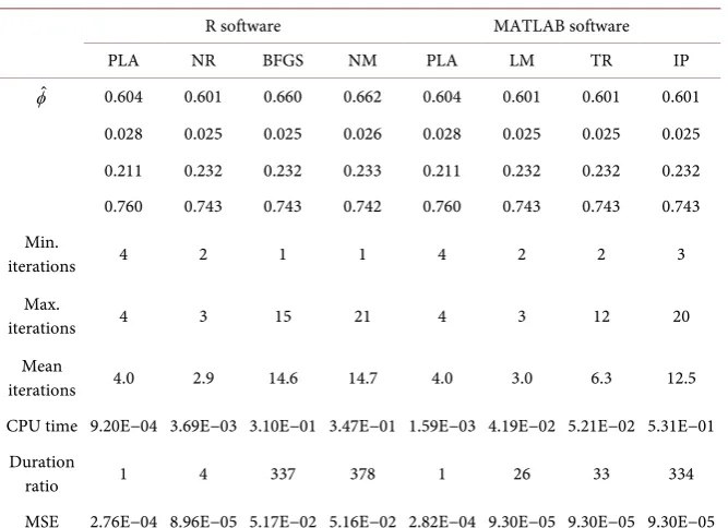
Table 4. Results for proportional initialisation of _β( )0 _,

3

r= , n=5000.

R software MATLAB software

PLA NR BFGS NM PLA LM TR IP

ˆ

φ 0.604 0.601 0.660 0.662 0.604 0.601 0.601 0.601

0.028 0.025 0.025 0.026 0.028 0.025 0.025 0.025 0.211 0.232 0.232 0.233 0.211 0.232 0.232 0.232 0.760 0.743 0.743 0.742 0.760 0.743 0.743 0.743 Min.

iterations 4 2 1 1 4 2 2 3

Max.

iterations 4 3 15 21 4 3 12 20

Mean

iterations 4.0 2.9 14.6 14.7 4.0 3.0 6.3 12.5

CPU time 9.20E−04 3.69E−03 3.10E−01 3.47E−01 1.59E−03 4.19E−02 5.21E−02 5.31E−01 Duration

ratio 1 4 337 378 1 26 33 334

MSE 2.76E−04 8.96E−05 5.17E−02 5.16E−02 2.82E−04 9.30E−05 9.30E−05 9.30E−05

algorithm is defined as the ratio between the mean computation time of this latter and the mean computation time of the PLA (therefore the duration ratio of the partial linear approximation algorithm always equals 1). The computation time depends on the computer used to perform the simulations while the duration ratio is computer-free and therefore more useful.

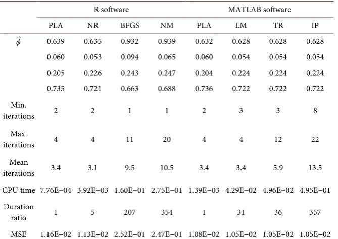
[image:12.595.207.541.367.609.2]

[image:13.595.207.542.91.328.2]

Table 5. Results for random initialisation of _β( )0

, r=3, n=50.

R software MATLAB software

PLA NR BFGS NM PLA LM TR IP

ˆ

φ 0.639 0.635 0.932 0.939 0.632 0.628 0.628 0.628

0.060 0.053 0.094 0.065 0.060 0.054 0.054 0.054 0.205 0.226 0.243 0.247 0.204 0.224 0.224 0.224 0.735 0.721 0.663 0.688 0.736 0.722 0.722 0.722 Min.

iterations 2 2 1 1 2 3 3 8

Max.

iterations 4 4 11 20 4 4 12 22

Mean

iterations 3.4 3.1 9.5 10.5 3.4 3.4 5.9 13.5

CPU time 7.76E−04 3.92E−03 1.60E−01 2.75E−01 1.39E−03 4.29E−02 4.96E−02 4.95E−01 Duration

ratio 1 5 207 354 1 31 36 357

MSE 1.16E−02 1.13E−02 2.52E−01 2.47E−01 1.08E−02 1.05E−02 1.05E−02 1.05E−02

Table 6. Results for random initialisation of _β( )0 _,

3

r= , n=5000.

R software MATLAB software

PLA NR BFGS NM PLA LM TR IP

ˆ

φ 0.603 0.600 0.839 0.841 0.603 0.600 0.600 0.600

0.028 0.025 0.067 0.036 0.028 0.025 0.025 0.025 0.211 0.232 0.244 0.252 0.211 0.232 0.232 0.232 0.760 0.743 0.689 0.712 0.760 0.743 0.743 0.743 Min.

iterations 3 2 1 1 3 3 3 8

Max.

iterations 4 4 15 20 4 4 12 31

Mean

iterations 4.0 3.4 13.2 13.4 4.0 3.4 6.5 14.1

CPU time 8.55E−04 4.40E−03 2.84E−01 3.31E−01 1.58E−03 4.30E−02 5.40E−02 5.34E−01 Duration

ratio 1 5 332 387 1 27 34 338

MSE 2.80E−04 9.40E−05 1.85E−01 1.75E−01 2.81E−04 9.55E−05 9.55E−05 9.55E−05

( )

(

)

2

(

)

2

0 0 0

1

1

ˆ ˆ ˆ

MSE , 1

r

j j j

r

φ φ θ θ β β

=

 

= _ − + − _

+ 

∑

 (20)

One can see that the MSE decreases when n (the total number of road crashes) increases. The PLA is at least as efficient as the other algorithms. It always converges to reasonable and acceptable parameter vector estimates and the estimate gets closer to the the true value as n increases.

[image:13.595.208.540.368.550.2]

produced by the PLA is relatively close to the true parameter vector and quite close to those of the other methods. More generally, all the compared methods have a MSE of order 2

10− . However the estimates produced by the BFGS and Nelder-Mead’s methods are very far from the true values (see Table 5). In the case of random initialisation, the MSE for Nelder-Mead’s and BFGS algorithms is 20 times greater than those of the other algorithms.

When n increases

(

n=5000

)

, the MSE of the PLA decreases from 2

10− to

4

10− . So the PLA is also efficient. Unsurprisingly, when n is very great the estimates produced by the other algorithms are closer to the true values than those of the PLA. This is expected because the other algorithms work with the exact gradient. However, the Nelder-Mead’s and BFGS algorithms produce estimates very far from the truth. Their MSE’s order is 2

10− (Table 4 and Table

6) while those of the PLA and the other methods are 4

10− .

To analyse the influence of the initial guess, we considered the mean number of iterations and the amplitude of the iterations (i.e. difference between the maximum and the minimum number of iterations). An increase in the am- plitude of iterations suggests a greater influence of the initial solution _φ( )0 _{. The}

results given in Tables 1-6 suggest that the PLA is stable and robust to initial guesses of the parameter being estimated. For the 6000 replications, the number of iterations needed by the PLA to converge lies between 2 and 4. In other words, setting the initial guess to 6000 different values chosen in the parameter vectors space does not disturb the PLA. This performance is as good as those of Newton- Raphson and Levenberg-Marquardt and by far better than those of BFGS, Nelder-Mead’s and Interior Point which have their number of iterations varying respectively from 1 to 15, 1 to 21 and 3 to 31.

As far as the computation time is concerned, it can be noticed that all the CPU time ratio are greater than 1 which means that none of the compared algorithms is faster than the PLA. On average, the PLA is 4 to 5 times quicker than Newton-Raphson, 239 to 345 times quicker than BFGS algorithm, 354 to 395 times quicker than Nelder-Mead, 27 to 31 times quicker than Levenberg- Marquardt, 33 to 39 times quicker than Trust region algorithms and 311 to 383 times quicker than Interior point algorithms. This can be an important factor when larger values of r are considered.

6. Real-Data Analysis

We apply the partial linear approximation algorithm to the data concerning the changes applied to road markings on a rural Nord Pas-de-Calais road (France)

four years after) on the marked area are given by Table 7.

Note that the number of fatal crashes (Fatal) decreased from four (in the before period) to one after the lay-out change. Indeed there were four accidents with at least one person killed in the period before the road works and one crash with at least one person killed in the period after. The number of slight crashes (no serious bodily injuries involved) recorded in the same period were more than halved. For the same lengths of time, on a portion of National Road 17 used as a control area, accident reports are the following.

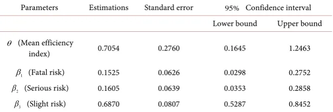
The values given in Table 8 are obtained by dividing, for each accident type, the number of crashes after the changes by the number of crashes before. On the whole, a decrease can be noted in comparison with the control area accident numbers between the 4-year period after the changes and the 4-year period before. All the algorithms can be applied to Table 7 and Table 8. Since the simulation results suggested that the partial linear approximation algorithm con- verges after a few iterations and remains steady, we only present the estimations related to the partial linear approximation algorithm (Table 9).

Parameters β1, β2 and β3 enable us to assess the risks for each type of

accident on the test area in the eight years when the road markings’ effects are studied. Estimated values βˆ1, βˆ2 and βˆ3 are respectively 0.1525, 0.1605 and 0.6870. These values suggest that in the eight years of road marking analysis, 15.25% of the crashes recorded in the test area were fatal, 16.05% were serious and 68.70% were slight as compared to the crashes recorded in the control area.

The estimated mean efficiency index

( )

_θˆ _{is 0.7054. It corresponds to an} average decrease in proportion of 29.46%= −

(

1 0.7054

)

×100% of the whole

Table 7. Crash data for experimental zone.

Accident data before Accident data after Total

Fatal Serious Slight Fatal Serious Slight

[image:15.595.205.538.558.591.2]

4 4 16 1 1 7 33

Table 8. Crash data for control zone.

Fatal Serious Slight

[image:15.595.210.539.624.735.2]

0.519 0.422 0.560

Table 9. Pas-De-Calais’s crash data using partial linear approximation algorithm.

Parameters Estimations Standard error 95% Confidence interval Lower bound Upper bound

θ (Mean efficiency

index) 0.7054 0.2760 0.1645 1.2463

1

β (Fatal risk) 0.1525 0.0626 0.0298 0.2752

2

β (Serious risk) 0.1605 0.0639 0.0353 0.2858

3

set of accidents in the test area as compared to the average trend in the control area. The mean effect significance for this type of lay-out may also be tested by using the confidence interval at the 95% level associated to parameter

θ

. This confidence interval reveals a bracket of values whose lower (resp. upper) bound is strictly superior to 0 (resp. 1). Indeed, as 1∈

[

0.1646,1.2463

]

, we cannot rule

out the hypothesis H0:θ =1 versus H1:θ ≠1 with a type-1 error of 5%.

Even if in the case studied here, we can notice a decrease in proportion of

(

)

29.46%= −1 0.7054 ×100% in the average accident number in the test area,

the above test shows that the mean efficiency index value is not significantly different from 1 to enable us to conclude that this type of road marking is efficient. In practice, an analysis according to periods, recorded data and control area should be carried out in order to get more appropriate conclusions.

7. Concluding Remarks

We propose in this paper, under assumptions, a principle of 2-block splitting of a constrained Maximum Likelihood (ML) system of equations linked to a parameter vector. We obtain analytical approximations of the components of the constrained ML estimator. The standard asymptotic errors are also obtained in closed-form.

We then build an iterative algorithm by initializing the first component of the parameter vector without inverting (at each iteration) the information matrix nor the Hessian matrix. Our partial linear approximation algorithm cycles through the components of the parameter vector and updates one component at a time. It is very simple to program and the constraints are integrated easily. To implement our algorithm, we use a particular version of the multinomial model of N’Guessan et al. [18] used to estimate the average effect of a road safety measure and the different accident risks when road conditions are improved. We prove that the assumptions are all satisfied and we obtain simple expressions of the estimators and their asymptotic variance. Afterwards, we give a practical version of our algorithm.

The numerical performance of the proposed algorithm is examined through a simulation study and compared to those of classical methods available in R and MATLAB software. The choice of these other methods is dictated not only by the fact that they are relevant and integrated in most statistical software but also by the fact that some need second order derivatives and others do not. The comparisons suggest that not only the partial linear approximation algorithm is competitive in statistical accuracy and computational speed with the best currently available algorithm, but also it is not disturbed by the initial guess.

The simulations results obtained on the particular model considered in this paper suggest that our algorithm may be extended to other families of multi- nomial models (such as the model of N’Guessan et al. [18]). Drawing our inspiration from [32], we may also prove the asymptotic strong consistency of the estimator obtained from our algorithm. This perspective will give a wider interest to our algorithm in the context of a large-scale use.

Acknowledgements

We thank the Editor and the anonymous referee for their remarks and sugges-tions which enabled a substantial improvement of this paper. This article was partially written while the second author was visiting the Lille 1 University (France).

References

[1] Hauer, E. (1997) Observational Before-After Studies in Road Safety Estimating the Effect of Highway Traffic Engineering Measures on Road Safety. Pergamon, Oxford. [2] N’Guessan, A., Essai, A. and Langrand, C. (2001) Estimation multidimensionnelle

des contrôles et de l’effet moyen d’une mesure de sécurité routière. Revue de Statis-tique Appliquée, 49, 85-102.

[3] Lord, D. and Mannering, F. (2010) The Statistical Analysis of Crash-Frequency Da-ta: A Review and Assessment of Methodological Alternatives. Transport Research Part A, 44, 291-305.

[4] Aitchison, J. and Silvey, S.D. (1958) Maximum Likelihood Estimation of Parameters Subject to Restraints. The Annals of Mathematical Statistics, 29, 813-828.

https://doi.org/10.1214/aoms/1177706538

[5] Crowder, M. (1984) On the Constrained Maximum Likelihood Estimation with Non-I.I.D Observations. Annals of the Institute of Statistical Mathematics, 36, 239-249. https://doi.org/10.1007/BF02481968

[6] Haber, M. and Brown, M.B. (1986) Maximum Likelihood Methods for Log-Linear Models When Expected Frequencies Are Subject to Linear Constraints. Journal of the American Statistical Association, 81, 477-482.

https://doi.org/10.1080/01621459.1986.10478293

[7] Lange, K. (2010) Numerical Analysis for Statisticians. 2nd Edition, Springer, Berlin.

https://doi.org/10.1007/978-1-4419-5945-4

[8] Li, Z.F., Osborne, M.R. and Prvan, T. (2003) Numerical Algorithms for Constrained Maximum Likelihood Estimation. ANZIAM Journal, 45, 91-114.

https://doi.org/10.1017/S1446181100013171

[9] Slivapulle, M.J. and Sen, P.K. (2005) Constrained Statistical Inference. Wiley, Ho-boken.

[10] Wang, Y. (2007) Maximum Likelihood Computation Based on the Fisher Scoring and Gauss-Newton Quadratic Approximations. Computational Statistics & Data Analysis, 51, 3776-3787. https://doi.org/10.1016/j.csda.2006.12.037

[11] Mkhadri, A., N’Guessan, A. and Hafidi, B. (2010) An MM Algorithm for Con-strained Estimation in a Road Safety Measure Modeling. Communications in Statis-tics - Simulation and Computation, 39, 1057-1071.

https://doi.org/10.1080/03610911003778119

for Log-Convex Models When Cell Probabilities Are Subject to Convex Constraints. The Annals of Statistics, 26, 1878-1893. https://doi.org/10.1214/aos/1024691361

[13] Matthews, G.B. and Crowther, N.A.S. (1995) A Maximum Likelihood Estimation Procedure When Modelling in Terms of Constraints. South African Statistical Journal, 29, 29-51.

[14] Liu, C. (2000) Estimation of Discrete Distributions with a Class of Simplex Con-straints. Journal of the American Statistical Association, 95, 109-120.

https://doi.org/10.1080/01621459.2000.10473907

[15] Ouellette, D.V. (1981) Schur Complement and Statistics. Linear Algebra and Its Applications, 36, 187-295. https://doi.org/10.1016/0024-3795(81)90232-9

[16] Zhang, F. (2005) The Schur Complement and Its Applications. Springer, Berlin.

https://doi.org/10.1007/b105056

[17] N’Guessan, A. and Langrand, C. (2005) A Covariance Components Estimation Procedure When Modelling a Road Safety Measure in Terms of Linear Constraints. Statistics, 39, 303-314. https://doi.org/10.1080/02331880500108544

[18] N’Guessan, A., Essai, A. and N’zi, M. (2006) An Estimation Method of the Average Effect and the Different Accident Risks When Modelling a Road Safety Measure: A Simulation Study. Computational Statistics & Data Analysis, 51, 1260-1277.

https://doi.org/10.1016/j.csda.2005.09.002

[19] N’Guessan, A. (2010) Analytical Existence of Solutions to a System of Non-Linear Equations with Application. Journal of Computational and Applied Mathematics, 234, 297-304. https://doi.org/10.1016/j.cam.2009.12.026

[20] N’Guessan, A. and Geraldo, I.C. (2015) A Cyclic Algorithm for Maximum Likelih-ood Estimation Using Schur Complement. Numerical Linear Algebra with Applica-tions, 22, 1161-1179. https://doi.org/10.1002/nla.1999

[21] Nelder, J.A. and Mead, R. (1965) A Simplex Algorithm for Function Minimization. Computer Journal, 7, 308-313. https://doi.org/10.1093/comjnl/7.4.308

[22] Broyden, C.G. (1970) The Convergence of a Class of Double-Rank Minimization Algorithms. Journal of the Institute of Mathematics and Its Applications, 6, 76-90.

https://doi.org/10.1093/imamat/6.1.76

[23] Fletcher, R. (1970) A New Approach to Variable Metric Algorithms. The Computer Journal, 13, 317-322. https://doi.org/10.1093/comjnl/13.3.317

[24] Goldfarb, D. (1970) A Family of Variable Metric Updates Derived by Variational Means. Mathematics of Computation, 24, 23-26.

https://doi.org/10.1090/S0025-5718-1970-0258249-6

[25] Shanno, D.F. (1970) Conditioning of Quasi-Newton Methods for Function Mini-mization. Mathematics of Computation, 24, 647-656.

https://doi.org/10.1090/S0025-5718-1970-0274029-X

[26] Waltz, R.A., Morales, J.L., Nocedal, J. and Orban, D. (2006) An Interior Algorithm for Nonlinear Optimization That Combines Line Search and Trust Region Steps. Mathematical Programming, 107, 391-408.

https://doi.org/10.1007/s10107-004-0560-5

[27] Levenberg, K. (1944) A Method for the Solution of Certain Problems in Least Squares. Quarterly of Applied Mathematics, 2, 164-168.

https://doi.org/10.1090/qam/10666

[28] Marquardt, D. (1963) An Algorithm for Least-Squares Estimation of Nonlinear Pa-rameters. SIAM Journal on Applied Mathematics, 11, 431-441.

[29] Byrd, R.H., Schnabel, R. and Shultz, G.A. (1988) Approximate Solution of the Trust Region Problem by Minimization over Two-Dimensional Subspaces. Mathematical Programming, 40, 247-263. https://doi.org/10.1007/BF01580735

[30] Varadhan, R. (2011) Alabama: Constrained Nonlinear Optimization. R Package Version 9-1.

[31] N’Guessan, A. and Truffier, M. (2008) Impact d’un aménagement de sécurité rou-tière sur la gravité des accidents de la route. Journal de la Société Française de Sta-tistiques, 149, 23-41.

[32] Geraldo, I.C., N’Guessan, A. and Gneyou, K.E. (2015) A Note on the Strong Con-sistency of a Constrained Maximum Likelihood Estimator Used in Crash Data Modelling. Comptes Rendus Mathematique, 353, 1147-1152.

8. Appendix

8.1. Proof of Lemma 1

Proof. Problem (3) is equivalent to maximizing function

(

φ λ,

)

=

( )

φ −λ φC

( )

 (21) where

λ

is the Lagrange multiplier. Any solution _φˆ _{must satisfy}

ˆ _ˆ

0 and 0, 1, , .

j j r φ _φ θ β   ∂ ∂  _{ =   = =} _∂  _{∂ }   _{ } 

  ₍₂₂₎

From assumption 3, system (22) is equivalent to

ˆ _{ˆ ˆ}

ˆ

0 and 0, 1, ,

j j

C

j r

φ _{φ φ}

λ

θ β β

    ∂ ∂ ∂  _{ = − = =}     _∂  _{∂  ∂ }   _{   }

  _{ (23)}

where _{λ λ φ}ˆ₌

( )

ˆ _{. After multiplication by} ˆ

j

β and summation on the index j, we get:

1 _ˆ 1 _ˆ

ˆ ˆ ˆ _0.

r r

j j

j j j j

C

φ φ

β λ β

β β = =  _∂  _∂  − =     _∂  _∂     

∑



∑

that is equivalent to

ˆ ˆ

ˆ_, ˆ ˆ_{,C 0.}

β φ

β λ β

β

∂  _{− =}

_∂ 

 



We obtain (6) by substitution of _λˆ _{in (23).} □

8.2. Proof of Theorem 2

Proof. Under conditions 6, Γφ is non singular and after some matrix mani-

pulations, we get

(

)

(

)

(

)

(

)

1 T 1

1

1 1 1

1 1 _{T 1}

1

1 1

1

,

W J C R

R C J R

J B J B U B

J

B U J B J

φ φ φ φ

φ

φ φ φ φ

φ φ φ φ φ φ

φ

φ φ φ φ φ τφ

− − − − − − − − ₋ − − − −  

Γ =  

−      ₋    =_{ } −    

where 1

2 1

,

n

R a C

φ

φ φ β −

− −

Σ

= _{is a scalar,}

(

1

)

1 2

1 1 1 1 T 1

, 1

n

B a V V V

φ

φ φ φ φ − φ φ φ φ

−

− − − − −

Σ

 

= _Σ − + Σ Σ _

 

is the inverse of B_φ,

(

)

(

1

)

1 ₂ 2

, , 1

n n

J B b a V

φ

φ φ φ φ φ −

− ₋

Σ

= + , is a scalar,

(

)

1 _{1 1}

,

n

J_φ τ_φ − =a−_{φ φ}Σ− , is a r×r matrix and Wφ =Jφ−1−J C R C Jφ−1 φT φ−1 φ φ−1 is the

(

1+ × +r

) (

1 r

)

asymptotic variance-covariance matrix of

φ

. We show that

( )

( )

( )

( )

T

1,1 2,1

2,1 2, 2

W W W W W φ φ φ φ φ   =      

where W_φ

( )

1,1 is a scalar and W_φ

( )

2, 2 is a r×r matrix. The asymptotic variance of _θˆ _{is given by W}

( )

_1,1

elements of W_φ

( )

2, 2 . After straightforward calculation, we get

( )

(

)

(

)

(

1

)

2 2

1 _{1 2} 2 _{, ,}

2 2 1,1 1 n n b a

W J B R J B

V φ

φ φ

φ φ φ φ φ φ φ

φ ξ − − − ₋ − Σ = − + and

( )

(

1

)

2

1 1 1 T 1

,

2, 2 n

W a C C C

φ

φ φ φ β − φ β β φ

−

− − − −

Σ

= Σ − Σ Σ

where T 1

V C

φ φ φ β

ξ _{= Σ}− _{. The results of Theorem 2 follow from a direct calculation.}

□

8.3. Proof of Corollary 2

Proof. Taking the second derivatives of the negative of  with respect to the components of

φ

and

λ

, we show that: λ22 λ θ2 0

∂ ∂

= =

∂ ∂ ∂

  _, 2

1 j λ β ∂ _{= −} ∂ ∂  _,

( )

(

)

( )

(

)

2 2 2.

2 2 2

1

n E Z y

E Z

θ θ _θ

∂ _{= − +} ∂ ₊  _,

( )

(

)

2 2 1 j j nz E Z

θ β _θ

∂ = −

∂ ∂ ₊

 _and

( )

(

)

(

( )

)

( )

(

)

(

( )

)

2 2 2

. 2.

2 2 2

2 2 2. 2 2 if 1 if 1

j j j

j

j k j k j k

y n z y z

j k

E Z E Z

n z z y z z

j k

E Z E Z

θ

β _θ

β β θ

θ  − + − =  +  ∂  =  ∂ ∂ _ − ≠  +  

for j, k=1,,r. Now, setting E y

( )

_.j =nβ_j, E y

( )

_2. =n E Zθ

( )

(

1+θE Z

( )

)

and γ =n

(

1+θE Z

( )

)

, we obtain the components of matrix J_φ as follows

( )

( )

( ) (

)

2 2 2 2

2

, , ,

, _j j, _jj j and _jk j k ,

j

z z z z

E Z n

U B B j k

n n nE Z nE Z

φ φ φ φ

γ γθ θγ

γ τ γ θ γβ   = = = _ + _ = ≠  

where Uφ,j (resp. Bφ,jj and Bφ,jk) are the components of vector Uφ (resp.

the elements of matrix Bφ). Using the last expressions of the elements of Uφ

and B_φ and after straightforward calculation, we show that

( )

1 1 1 T

2, 2

W

n

φ =γ−Σ −φ− ββ and then, we deduce the expression of σ βˆ2

( )

ˆj

given by corollary 2. In the same way, we obtain

( )

1,1 2

_{( )}

2 n

W

n t E Z

φ

φ

θ θ

γ

= −

where 2

( )

2

( )

2_ˆ

( )

2

t_φ =_n E Z _{ } n E Z +θγ E Z _. Using the last expression of t_φ, we get the expression of 2

( )

_ˆ

ˆ

σ θ . □

Submit or recommend next manuscript to SCIRP and we will provide best service for you:

Accepting pre-submission inquiries through Email, Facebook, LinkedIn, Twitter, etc. A wide selection of journals (inclusive of 9 subjects, more than 200 journals)

Providing 24-hour high-quality service User-friendly online submission system Fair and swift peer-review system

Efficient typesetting and proofreading procedure

Display of the result of downloads and visits, as well as the number of cited articles Maximum dissemination of your research work