Is India Ready for Inflation Targeting?

Munich Personal RePEc Archive

Is India Ready for Inflation-Targeting?

Sen Gupta, Abhijit and Sengupta, Rajeswari

Asian Development Bank, Indira Gandhi Institute of Development

Research

4 June 2014

Online at

https://mpra.ub.uni-muenchen.de/57463/

Is India Ready for Inflation Targeting?1

Abhijit Sen Gupta*

Asian Development Bank (ADB)

Rajeswari Sengupta**

Indira Gandhi Institute of Development Research (IGIDR)

Abstract

In this paper we analyze whether the current macroeconomic environment in India is suitable for implementation of inflation targeting as a monetary policy strategy, in light of the recommendation of the Urjit Patel Committee Report. Our results indicate that historically the Reserve Bank of India has given more importance to inflation compared to output growth and exchange rate changes in its monetary policy conduct and that in recent times there has been an increased emphasis on monetary independence thereby comfortably placing the RBI on a path to move towards inflation targeting. However we also find factors, that are traditionally outside the control of monetary policy, do exert a strong impact on aggregate prices in India thereby making the choice of nominal anchor a tricky one. Furthermore, the success of monetary policy in containing inflation is found to be crucially contingent on an appropriate fiscal policy as well.

JEL Classification: E43; E52; E58

Keywords: Reserve Bank of India, Monetary Policy, Taylor Rule, Financial trilemma, Inflation, Nominal anchor, Fiscal deficit

1

The views expressed in this paper are those of the author/s and do not necessarily reflect the views and policies of the Asian Development Bank (ADB) or its Board of Governors or the governments they represent.

*

Abhijit Sen Gupta, India Resident Mission, Asian Development Bank. 4 San Martin Marg, Chanakyapuri, New Delhi – 110021. Email: [email protected]. Phone: +91 11 24194284.

**

1. Introduction

In January 2014, the Expert Committee to Revise and Strengthen Monetary Policy Framework

under the chairmanship of Dr. Urjit Patel (henceforth Urjit Patel Committee Report (UPCR)) made

several important recommendations related to the conduct of monetary policy in India. These

include (a) Using the Consumer Price Index (CPI) inflation as the nominal anchor for monetary

policy communication; (b) moving towards an inflation targeting regime over the next two years

with a target of 4% within a band of ±2%; and (c) setting up a five member Monetary Policy

Committee, which will be responsible for making policy decisions, and be held accountable in

case of failure to meet the nominal target.

In India, there has been a long-standing debate on the benefits and costs involved with a move

towards inflation targeting. HPEC (2007), also known as Percy Mistry Committee Report, strongly

advocated a move towards inflation-targeting pointing out associated benefits including fiscal

stability and low output volatility. It also argued that an institutional commitment to predictable and

low inflation would reduce risks from capital flight as value of the Rupee would be maintained in

real terms and expectations about its future values would be stable. While it advocated the use of

Consumer Price Index (CPI) inflation as the nominal target, it pointed out the necessity to cease

subsidization of key prices and intervention in the commodity markets through price measures.

Similarly, Planning Commission (2011) argued for reorientation of monetary policy towards price

stability or low and stable inflation, although the report does highlight the deflationary cost

associated with bringing down inflation from high levels and to build credibility for a central bank

that has lacked inflation fighting credentials. Shah (2014) argues that every currency needs a

nominal anchor as otherwise a country might end up printing too much ‘fiat money’, and that a

foreign currency and CPI basket are the possible choices for nominal anchor. Of these, pegging

to a foreign currency results in loss of monetary independence, and can lead to costly crises as

witnessed in East Asia in 1997. In contrast, targeting inflation provides a durable long-term

solution.

In sharp contrast, Subbarao (2009) points out that “… inflation-targeting is neither desirable nor

practical in India for a number of reasons.” These include (a) the need of a central bank of a

developing country being guided by price stability, financial stability and growth; (b) food items

continue to be vulnerable to supply shocks, especially because of vagaries of monsoon, and are

beyond the ambit of monetary policy; (c) inefficient transmission mechanism due to large fiscal

deficits, presence of administered prices and interest rates and illiquid private bond market; and

In the aftermath of the UPCR, a number of articles have questioned the desirability and efficacy

of inflation targeting in India. Nachane (2014) argues that inflation targeting regime, with an

overwhelming desire to manage inflation, could have an adverse effect on a number of macro

financial variables including exchange rate management, fiscal policy and financial stability.

The rest of the paper is structured as follows. Section 2 describes the main recommendations of

the Urjit Patel Committee Report. In Section 3 we evaluate whether India is indeed amenable to

the implementation of an inflation targeting (IT) regime by estimating a Taylor Rule for India.

Section 4 highlights some of the key issues that policymakers will have to deal with if India moves

on the path of inflation targeting regime. Finally Section 5 concludes with a summary of the main

messages of the paper.

2. Key Highlights of the UPCR

The UPCR argues for the adoption of an inflation targeting regime, under which the objective is to

achieve the inflation target on average over the business cycle. The report points out that by

predominantly focusing on price stability, an inflation targeting regime anchors inflation

expectations, improves overall macroeconomic stability, and enhances growth prospects in the

medium run. At the same time, an inflation targeting regime allows the inflation to deviate from

the target in the short run to accommodate growth concerns.

The UPCR favours domestic inflation as the nominal anchor over other historically used

measures such as the exchange rate and monetary aggregates. While using the former as the

nominal anchor involves relinquishing monetary policy independence and makes the monetary

policy framework susceptible to speculative attacks and currency crisis, the use of latter can be

undermined by instability and loss of predictability of the demand for money, thereby discrediting

accountability and communication when targets are missed.

In contrast, using domestic inflation as the nominal anchor makes price stability the unambiguous

and sustainable objective upon which the private sector can anchor future inflation expectations.

It also has the advantage of being simple and easily communicable, and thereby well understood

by the public. However, focusing exclusively on inflation also has its disadvantages. First, certain

components of inflation such as food and fuel cannot be directly controlled by the monetary

policy. Second, the long and variable lags in monetary policy transmission makes targeting

inflation a medium term approach. Finally, overarching emphasis on achieving the targeted

The UPCR favours the use of the all India Consumer Price Index Combined inflation against the

traditional Wholesale Price Index (WPI) inflation as the inflation metric. This is primarily driven by

the CPI Combined index capturing price movements in service sectors, which accounts for nearly

two-thirds of GDP. This index is also subject to marginal revisions, critical for policy formulations

as large revisions result in uncertainty in the assessment of inflation conditions. Moreover, CPI

Combined has the advantage of capturing more accurately the true inflation that the consumer

faces in the retail market.

On the choice of headline versus core inflation, UPCR shows a preference for headline inflation,

including food and fuel inflation. The latter tends to have an important bearing on aggregate

inflation expectations as it gets manifested in the inflation of other items with a lag. Moreover,

UPCR also notes that shocks to food and fuel inflation have a larger and more persistent impact

on inflation expectations compared to non-food inflation. At the same time, the construction of the

consumption basket makes it difficult to completely isolate the impact of food and fuel inflation.

Exclusion of food and fuel inflation results in discarding around 57 percent of the consumption

basket. However, even with the exclusion of food and fuel inflation, other components of the

consumption basket such as transport and communication are impacted by change in diesel and

petrol prices, and further segregation is not possible as item level disaggregated price index is not

available. For these reasons the UPCR focuses on CPI Combined inflation recognising that a part

of the inflation would be outside the ambit of the monetary policy.

In selecting a numerical target, the UPCR relies on both comparator emerging market economies

as well as India’s historical experience. The literature points out that while in advanced

economies an inflation rate of 1 percent to 3 percent is viewed as acceptable, in emerging

markets, acceptable inflation rate tends to be around 4 percent to 5 percent. Using empirical

methods, the report finds that during the period from 2003-04Q3 to 2006-07Q1, when India’s

output gap was fairly close to zero, CPI inflation averaged 4 percent. Similarly using quarterly

data from 1996-97 to 2012-13, the report finds CPI-Combined inflation of above 6.2 percent is

inimical to growth. Based on this analysis, UPCR recommends that the nominal anchor should be

set at 4 percent with a band of ±2 percent around it. The UPCR stipulates a period of two years to

achieve the inflation target. This is based on the costs imposed by high inflation in the form of real

effective exchange rate (REER) appreciation, high current account deficit, erosion of financial

savings and resultant decline in financial saving and investment that hampers growth.

The UPCR also lays down some of the key changes in the institutional framework required to

undertake a successful transition to an inflation targeting regime. A key precondition is to follow a

transmission. The report also recommends the elimination of various administered prices, wages

and interest rates that hinder the smooth transmission of monetary policy.

3. Taylor Rule Estimation

In order to find out whether the macroeconomic environment in India is indeed ready for the

implementation of an inflation targeting framework, it is also important to understand the relative

weights placed by the RBI on varying policy objectives within the framework of a conventional

monetary policy rule. The RBI has mostly followed a pragmatic approach towards monetary policy

responding to the state of the economy in a seemingly discretionary manner best outlined by a

former Deputy Governor of RBI as follows, “….the overall objective has had to be approached in

a flexible and time variant manner with a continuous rebalancing of priority between growth and

price stability, depending on underlying macroeconomic and financial conditions” (Mohan 2006).

Since Indian monetary policy is conducted in a highly discretionary manner, and somewhat

non-transparently, our empirical analyses using past time-series data can provide important insights

into the “revealed preferences” of the RBI.

Theoretical studies that derive optimal monetary policy rules, and empirical studies that

investigate their use in practice, are now commonplace in the literature (e.g. Taylor, 1993;

Clarida, Gali, Gertler, 2000; Woodford, 2001). Taylor (1993) formulated a policy rule by which the

U.S. Federal Reserve adjusts the policy rate in response to past inflation and output gap (actual

less potential output). Many studies subsequently applied and developed this class of policy rule

to examine the behavior of central banks in industrialized countries (e.g., Clarida et al., 2000), as

well as to emerging economies. In what follows we investigate whether the RBI’s seemingly

discretionary approach can in practice, be described by a Taylor-type rule in the same spirit as

Hutchison, Sengupta and Singh (2010), Mohanty and Klau (2005) and Virmani (2004).

3.1. Brief background of Indian Monetary Policy

The monetary policy framework in India and the associated operating procedure have evolved

over time. The structural reforms and financial liberalization of the 1990s marked a paradigm

shift. Swings in capital flows and rising volatility of the exchange rate made it difficult to target

monetary aggregates. Interest rates and the exchange rate began to be increasingly market

determined. The RBI was able to move away from direct instruments to indirect market-based

instruments in its liquidity management operations. By 1997, Cash Reserve Ratio (CRR) and

Statutory Liquidity Ratio (SLR) were brought down. RBI broadly followed the monetary targeting

In April 1998, RBI adopted a ‘multiple indicator approach’ with greater emphasis on interest rate

and exchange rate channels for monetary policy transmission, relative to quantity instruments.

Under the multiple indicator approach, which is currently in use, a number of variables such as

money, credit, output, merchandise trade, capital flows and fiscal situation as well as interest

rates, rates of return in different financial markets, inflation rate and exchange rate are analyzed

for drawing monetary policy inferences.

The RBI also introduced the Interim Liquidity Adjustment Facility (ILAF) in April 1999, under which

liquidity injection was done at the bank rate and liquidity absorption was through fixed reverse

repo rate. The ILAF gradually transitioned into a full-fledged liquidity adjustment facility (LAF) that

was operated through overnight fixed rate repo and reverse repo from November 2004 onwards.

The LAF helped to develop interest rate as an instrument of monetary transmission.

In the process, two major weaknesses were revealed in the functioning of monetary policy. First

was lack of a single policy rate. The operating policy rate alternated between repo and reverse

repo rates depending upon the prevailing liquidity condition. In a surplus liquidity condition, the

operating policy rate was the reverse repo rate, while in a deficit liquidity situation it was the repo

rate. Second was the lack of a firm corridor. The overnight interest rates dipped below the reverse

repo rate in surplus conditions and rose above the repo rate in deficit conditions. Moreover,

overnight call rates became unbounded under occasional liquidity stress. Thus, more often the

overnight interest rate remained outside the corridor.

In May 2011, the RBI announced a revised monetary policy operating procedure based on the

recommendations of a committee constituted for the purpose. The new operating procedure

retained the essential features of the LAF framework with a few key modifications.

• First, the weighted average overnight call money rate was explicitly recognized as the

operating target of monetary policy.

• Second, the repo rate was made the only one independently varying policy rate.

• Third, a new Marginal Standing Facility (MSF) was instituted under which scheduled

commercial banks (SCBs) could borrow overnight at their discretion up to 1% of their

respective NDTL (banks’ net demand and time liabilities) at 100 basis points above the

repo rate.

• Fourth, the revised corridor was defined with a fixed width of 200 basis points. The repo

rate was placed in the middle of the corridor, with the reverse repo rate 100 basis points

below it and the MSF rate 100 basis points above it.

The new operating framework with the modified LAF presupposes the dominance of the interest

rate, it should immediately impact the overnight interest rate, which is the operational rate and

then transmit through the term structure of interest rates as well as bank lending rates.

3.2. Data and Empirical Methodology

Against the above background we split our sample into sub-periods based on major changes in

the monetary policy framework. We use quarterly data from 1990 to 2013 and estimate the Taylor

rule for three separate windows: 1990Q1-1998Q1; 1998Q2-2004Q3 and 2004Q4-2013Q2. The

break in 1998 reflects the adoption of the multiple indicator approach and the one in 2004

coincides with implementation of the LAF. We first estimate a standard Taylor rule based on the

hypothesis that the RBI reacts to both the output gap and inflation while setting the policy interest

rate.2 We also augment the standard Taylor Rule by incorporating exchange rate change as a third objective, given its significance in previous work (Hutchison, Sengupta and Singh, 2010;

Mohanty and Klau, 2005):

(1)

Where, is the nominal interest rate, is the output gap (deviation of actual output from

potential output), is the inflation rate at time t (assuming a constant inflation target such that

the target is subsumed in the constant term of the equation) and is the first difference of the

log of nominal exchange rate. According to the Taylor Rule, the estimated coefficients of equation

(5), , and should all have positive signs. The rule thus implies that interest rate should go

up when actual output exceeds the potential output, when inflation goes up or when exchange

rate depreciates. We estimate equation (5) for the three sub-sample periods mentioned above.

For the empirical estimation, we use the overnight call or money market rate for the policy rate.

As regards the potential output level, unlike developed countries, in India there are no official

measures. We derive the output gap using the standard Hodrick-Prescott (HP) filter for measuring

trend output and taking the residual of HP filter. We use the Index of Industrial Production (IIP) as

a measure of output.3 We calculate year-on-year inflation using percentage changes in the

2

objectives at the same time such as output gap, inflation rate and exchange rate and it also helps estimate the extent of persistence in the monetary policy. Hence, in order to assess the importance assigned by the RBI to inflation as compared to other objectives of monetary policy, we consider estimating the Taylor Rule an appropriate empirical mechanism.

3

Ideally, we could have liked to use GDP to calculate the output gap. However, we are constrained by the unavailability of quarterly data on GDP for India before 1996-97. Hence, we use quarterly data for IIP which is available from the start of our sample period; it reflects the movement in the industrial sector, which accounts for 25% to 30% of the Indian

Wholesale Price Index (WPI) as well as the Consumer Price Index for Industrial Workers

(CPI-IW) given that the latter has received significant policy attention in recent times especially in light

of the UPCR.

Prior to estimations, we conduct unit root tests (Augmented Dickey-Fuller, Phillips-Perron,

Elliott-Rothenberg-Stock and Kwiatkowski-Phillips-Schmidt-Shin tests) and results suggest presence of

unit root in the exchange rate series in levels, but we find that the first difference of the series is

stationary. Accordingly, we use first difference of the nominal exchange rate as specified in

equation (5) above. We also run the Durbin Watson and Breusch-Godfrey tests that reveal the

presence of serial correlation and the Breusch-Pagan/Cook-Weisberg test that shows presence

of heteroskedasticity in error terms. Accordingly, we estimate our baseline model given in

equation (5) using ordinary least squares regression with Newey-West variance-covariance

matrix, in order to correct for both autocorrelation and heteroskedasticity. We have also

de-seasonalized the series using the Census X12 procedure.

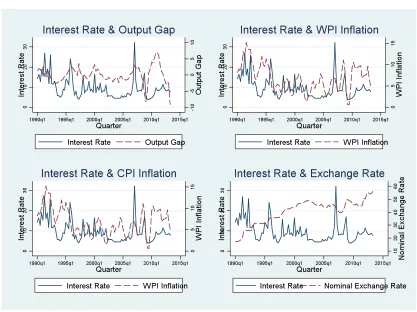
Figure 1: Relationship between Interest Rate and Key Macroeconomic Variables

Source: Database on Indian Economy and Authors’ Calculations

The Woodford (2001) version of the Taylor Rule for an open economy expresses the policy

rate. Hence we further augment equation (1) by adding lagged interest rate in order to capture

inertial in optimal monetary policy or interest rate persistence.

(2)

This equation is also estimated for three sub-periods. Figure (1) above shows the evolution of the

output gap, inflation (WPI and CPI), and nominal exchange rate series along with overnight

interest rate during the sample period.

3.3. Discussion of results

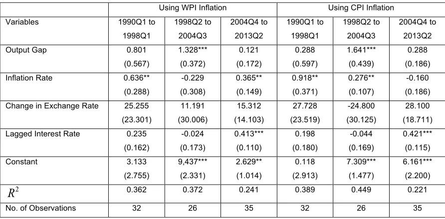
The results of estimating equations (1) and (2) are given in Tables (1) and (2) respectively. The

first three columns of Table (1) show the results for estimating equation (1) using WPI to measure

inflation whereas the last three columns show results, with inflation calculated using CPI.

Columns 1 and 4 truncate the sample at 1998Q1, and columns 2 and 5 truncate the sample at

2004Q3. Each of these truncations represents a plausible break point from the perspective of

changes in conduct of Indian monetary policy, as outlined in section 3.1 above. All the estimated

coefficients whenever significant have the expected positive sign as predicted by theory implying

that RBI has on average raised interest rate when output has been above its potential level or

inflation has gone up or the nominal exchange rate change has been positive i.e. exchange rate

has depreciated.

Table (2) shows results for estimating the baseline Taylor Rule with lagged interest rate. Results

are similar to Table (1) and we also find that interest rate has exhibited higher persistence in the

final sub-period i.e. the inertia in monetary policy has been much higher in recent times.

It can be further seen from the table that output gap is statistically significant only during

1998Q2-2004Q3 irrespective of the index used to measure inflation, implying that the RBI has not always

been consistently responsive to output growth per se. The effective responsiveness to output gap

depends on adjusting for the magnitude of lagged interest rate coefficient (Hutchison, Sengupta,

Singh, 2010). Clearly the interest rate persistence does not seem to have affected output gap

during the period 1998Q2-2004Q3 as shown the similar magnitude of raw coefficients of output

gap across the two tables.

WPI inflation seems to have been relatively important during the first and last sub-periods

whereas CPI inflation has been consistently significant during 1990Q1-2004Q3 but not in the

most recent period. The estimated coefficient of CPI inflation is greater than 1 in both Table 1 and

and Table 2 (when adjusted for the lagged interest rate) for the period 1990Q1-1998Q1 indicating

of the WPI inflation coefficient though close but never exceeds 1 even when adjusted for interest

rate persistence. Thus, historically the central bank seems to have put greater emphasis on

inflation rate compared to output gap.

Table 1: Taylor Rule Estimation: Without Interest Rate Persistence

Using WPI Inflation Using CPI Inflation Variables 1990Q1 to

1998Q1 1998Q2 to 2004Q3 2004Q4 to 2013Q2 1990Q1 to 1998Q1 1998Q2 to 2004Q3 2004Q4 to 2013Q2 Output Gap 1.104

(0.651) 1.314*** (0.333) 0.008 (0.179) 0.424 (0.711) 1.608*** (0.386) 0.215 (0.181) Inflation Rate 0.806***

(0.280) -0.221 (0.291) 0.452** (0.215) 1.108*** (0.314) 0.270** (0.097) -0.218 (0.312) Change in Exchange Rate 34.957

(23.715) 9.177 (26.406) 6.703 (21.604) 36.171 (24.447) -27.503 (29.909) 22.611 (24.482) Constant 4.252

(2.709) 9.210*** (1.407) 5.631*** (1.617) 0.445 (3.181) 6.981*** (0.693) 10.266*** (3.192) 0.327 0.372 0.073 0.364 0.448 0.046

No. of Observations 32 26 35 32 26 35 Note: Robust Newey West Standard errors in parentheses. ***, **, and * denote significance at the 1 percent, 5 percent, and 10 percent levels, respectively.

Source: Authors’ calculations

Table 2: Taylor Rule Estimation: With Interest Rate Persistence

Using WPI Inflation Using CPI Inflation Variables 1990Q1 to

1998Q1 1998Q2 to 2004Q3 2004Q4 to 2013Q2 1990Q1 to 1998Q1 1998Q2 to 2004Q3 2004Q4 to 2013Q2 Output Gap 0.801

(0.567) 1.328*** (0.372) 0.121 (0.172) 0.288 (0.597) 1.641*** (0.439) 0.288 (0.186) Inflation Rate 0.636**

(0.288) -0.229 (0.308) 0.365** (0.149) 0.918** (0.371) 0.276** (0.107) -0.160 (0.186) Change in Exchange Rate 25.255

(23.301) 11.191 (30.006) 15.312 (14.103) 27.728 (23.519) -24.800 (30.125) 28.100 (18.711) Lagged Interest Rate 0.235

(0.162) -0.024 (0.173) 0.413*** (0.110) 0.198 (0.180) -0.044 (0.169) 0.421*** (0.115) Constant 3.133

(2.755) 9,437*** (2.331) 2.629** (1.014) 0.118 (2.913) 7.309*** (1.477) 6.161*** (2.200) 0.362 0.372 0.241 0.389 0.449 0.221

No. of Observations 32 26 35 32 26 35 Note: Robust Newey West Standard errors in parentheses. ***, **, and * denote significance at the 1 percent, 5 percent, and 10 percent levels, respectively.

However the magnitude of the inflation coefficients for both indices has dramatically gone down

over the years—in fact for WPI inflation, both with and without interest rate persistence taken into

account, the coefficients have almost halved between the first and last sub-periods. Also while

WPI inflation is statistically significant at the 5% confidence level during 2004Q4-2013Q2, not

only is CPI inflation not significant, its coefficient turns negative. A plausible reason for the

insignificant coefficient on CPI inflation in the last sub-period could be the widening gap between

CPI and WPI inflation, especially during the latter half of this sub-period, owing to a surge in food

prices. Food inflation affects WPI and CPI inflation in a disproportionate manner due to the higher

weight of food items in the CPI basket compared to the WPI basket. Another likely reason could

be that the central bank was responding to the rise in inflation during the second half of the

sub-period only in an incremental and lagged manner.

Going purely by WPI inflation, coefficient magnitudes and statistical significance, it seems that the

though the relative importance assigned to inflation has diminished during the second sub-period

(1998Q2-2004Q3), it has been somewhat recovered in recent times. If we consider CPI inflation

however, the importance assigned to it seems to have declined over the sample period. Hence,

when it comes to weight assigned by the RBI to inflation in monetary policy, clearly the index of

measurement matters.

We further find that in line with the RBI’s own policy stance, exchange rate movements do not

constitute a systematically important determinant of its monetary policy conduct over the entire

sample period-a result also consistent with earlier findings in Hutchison, Sengupta and Singh

(2010). In none of the sub-periods do we find the estimated coefficients of exchange rate change

to be statistically significant, irrespective of whether we take into account inertia in monetary

policy.

Overall, our results seem to indicate that inflation matters more than output gap if we are to use

Taylor Rule to understand Indian monetary policy, there has been greater sensitivity to WPI

inflation in recent times compared to CPI, exchange rate changes do not seem to play a crucial

role and post-2004 conduct of monetary policy seems to have changed in the direction of greater

inertia.

A comparison of the interest rate predicted by specifications outlined in Table (2) with the actual

interest rate yields interesting results. In the case of CPI inflation, during the period 1990Q1 to

1998Q1, the Taylor Rule predicted rate was on average around 3 percentage points lower than

the prevailing interest rates. During the second sub-period, we find that on average prevailing

interest rates were in line with the rates predicted by the Taylor Rule. Finally, in the third

sub-period we find monetary policy to be tad loose with interest rates predicted by the Taylor Rule

4. Issues under an Inflation Targeting Regime

The move towards an inflation targeting regime marks a significant departure from the traditional

multiple indicator approach. This would entail the central bank confronting a number of issues.

Below, we describe a few key challenges that the RBI would have to overcome as it moves

towards an inflation targeting regime. These include (a) managing the impossible trinity; (b)

deciding upon the inflation metric to use as a target; (c) determining the appropriateness of the

numerical target; and (d) assessing the impact of fiscal dominance. We understand that this is not

an exhaustive list of the challenges being faced by a central bank as it aims to undertake a

transition to an inflation targeting regime.4 Mahajan et al.(2014) highlight a number of other issues including absence of well-developed capital markets and accurate forecasting techniques.

4.1 How to manage the impossible trinity?

A fundamental contribution of the Mundell-Fleming framework is the impossible trinity, which

states that a country may choose any two, but not all of the following three goals at the same

time: monetary independence, exchange rate stability and capital account openness or financial

integration (Aizenman, et al., 2008). Under this standard framework of the impossible trinity, given

India’s enhanced integration with global capital markets, there would be a tension between

monetary independence and exchange rate management.5 The adoption of an inflation targeting mechanism would result in the central bank relinquishing exchange rate management in favour of

greater monetary independence. This could prove to be perilous given the sharp increase in

volatility of capital flows in recent years. The central bank has grappled with the impossible trinity

over the last several years. Below we use empirical methods to describe briefly India’s

experience with impossible trinity using quarterly data from 2000 Q1 to 2013 Q4.6

Monetary Independence (MI)

Following Aizenman et al. (2010), the extent of monetary independence is measured as the

inverse of the quarterly correlation of the interest rates between India and the US. The quarterly

indices are calculated using weekly 3-month Treasury Bill yields for India and the US. The index

of Monetary Independence is given by

(3)

4

For instance, in India the government bond market is much less developed compared to the same in OECD countries or for that matter other major emerging economies and the corporate bond market is even more illiquid-both of which pose significant constraints in an effective monetary transmission which in turn might hamper the successful implementation of an inflation targeting strategy. See Anand and Sengupta (2014), Banerji et. al (2012) and Mitra (2009) for a detailed discussion of the Indian corporate debt market.

5

The Impossible Trinity or the Trilemma points out that that it is impossible to attain monetary policy independence, exchange rate stability and capital market integration simultaneously. Only two of the three objectives can be obtained at a particular point in time.

6

where corr   (iIND,iUS), refers to the correlation of the interest rates over a quarter and provides evidence on co-movement of domestic and foreign interest rates. A higher value of the index

refers greater degree of monetary independence.

Exchange Rate Stability (ERS)

We use the methodology introduced by Frankel and Wei (1994) to create an index of exchange

rate stability. The degree of influence that major global currencies have on Indian Rupee can be

estimated using the following estimation model

(4)

Where is the exchange rate of currency i against the numèraire currency, which in this case

is the Swiss franc where currency i can be the US Dollar, Japanese Yen and the Euro. Under this

estimation, which is the estimated coefficient on the rate at which currency i depreciates

against the numèraire currency indicates the weight of currency i in the basket. In the case where

the currency under observation is pegged to a particular currency or a basket of currency we will

have or for i currencies that are a part of the basket. Moreover, pegging to an

individual or a basket of currencies implies a higher goodness of fit. We apply the estimation over

a quarter and take the goodness of fit, or the adjusted R2 as the measure of exchange rate stability. A higher R2 indicates greater pegging to an individual or a basket of currencies.

Capital Account Openness (KO)

The index of capital account openness is based on a de facto measure of openness, as it is the

actual volume of flows that creates a conflict between monetary independence and exchange rate

stability as opposed to controls governing the movement of capital. The index of capital account

openness, KO, is based on net capital flows, and is constructed as the ratio of absolute value of

net capital flows to GDP.

(5)

To make the indices comparable, all the indices are normalized to lie between 0 and 1.7

7

The validity of trilemma framework in India is estimated by testing whether the weighted sum of

the three trilemma policy variables adds up to a constant – here set to be 2.8

(6)

Using the methodology outlined in Bai and Perron (2003) to identify structural breaks, we find that

the exchange rate regime in India can be classified into four distinct phases. These are: Phase I:

2000 Q1 to 2005 Q3; Phase II: 2005 Q4 to 2008 Q3; Phase III: 2008 Q4 to 2011 Q3 and Phase

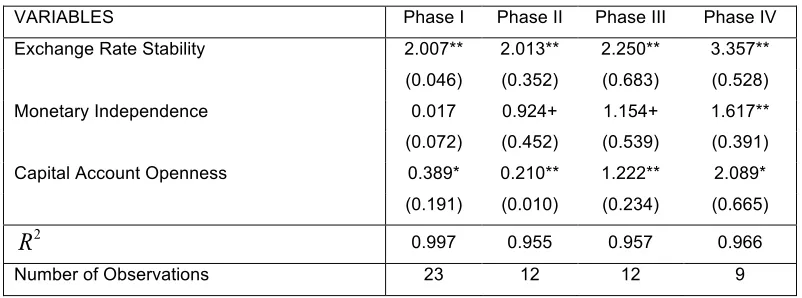
IV 2011 Q3 to 2013 Q4. We find that the overall fit is extremely high with R2 being above 0.93 across all the specifications, implying that the linear trilemma specification is a good

approximation for India (Table (3)). While the estimates for exchange rate stability and capital

account openness are significant across all the specifications, it is not the case with monetary

independence.

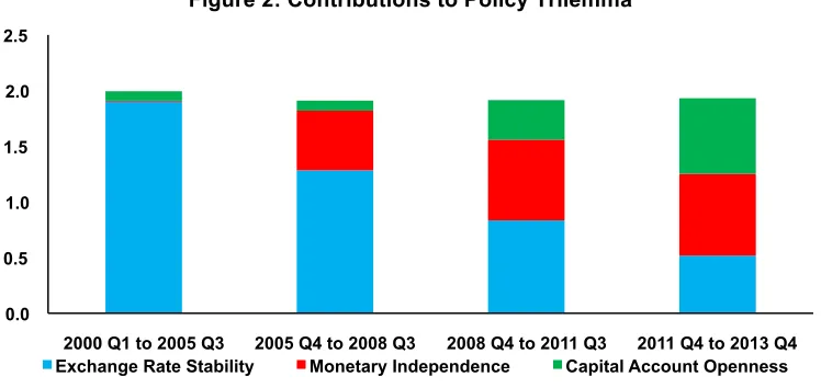
To obtain the weight assigned by the policymaker to the three different policy orientations of the

trilemma we multiply the coefficients with the average for each phase (Table 4). The results are

outlined in Figure 2.

Table 3: Testing the Validity of the Trilemma Framework

VARIABLES Phase I Phase II Phase III Phase IV

Exchange Rate Stability 2.007** 2.013** 2.250** 3.357**

(0.046) (0.352) (0.683) (0.528)

Monetary Independence 0.017 0.924+ 1.154+ 1.617**

(0.072) (0.452) (0.539) (0.391)

Capital Account Openness 0.389* 0.210** 1.222** 2.089*

(0.191) (0.010) (0.234) (0.665)

0.997 0.955 0.957 0.966

Number of Observations 23 12 12 9

Robust standard errors in parentheses ***p<0.01, * *p<0.05, *p<0.1 Source: Authors’ calculations

8

Table 4: Average Values of the Trilemma Indices

VARIABLES Phase I Phase II Phase III Phase IV

Exchange Rate Stability 0.947 0.638 0.371 0.154

Monetary Independence 0.499 0.580 0.629 0.454

Capital Account Openness 0.218 0.429 0.291 0.325

Source: Authors’ calculations

It is clearly evident that across the phases there has been a decline in the weight assigned to

exchange rate stability. In Phase I exchange rate stability was the overwhelmingly dominant

objective of the policymakers. However, by Phase IV the weight assigned to this objective had

dropped to a third of that in Phase I. The Rupee appreciated by nearly 17 percent between March

2009 and April 2010. Similarly, between August 2011 and December 2011, the Rupee

depreciated by 19 percent on the back of a widening current account deficit and weak capital

inflows. The Rupee witnessed heightened volatility in 2013 as well. A high current account deficit

and signals of tapering of the quantitative easing by the Federal Reserve in the USA resulted in

the Rupee depreciating by 21 percent between May and August 2013. The various policy

measures introduced to curb the current account deficit and enhance capital inflows helped the

Rupee strengthen by 11 percent by November 2013.

Figure 2: Contributions to Policy Trilemma

Source: Authors’ calculations

In contrast there has been a steady increase in both capital account openness and monetary

independence. The rise in capital account openness has been driven by India’s increased

integration with global capital markets. While gross capital flows as a percentage of GDP

increased from 21 percent in 2000-01 to 52.1 percent in 2013-14, net capital flows rose from 1.9

percent to 2.6 percent.

0.0 0.5 1.0 1.5 2.0 2.5

2000 Q1 to 2005 Q3 2005 Q4 to 2008 Q3 2008 Q4 to 2011 Q3 2011 Q4 to 2013 Q4

At the same time, the central bank pursued a more independent monetary policy. After the initial

softening of monetary policy to stimulate growth, the RBI started tightening the monetary policy

from March 2010 in response to high and persistent inflation. This was in contrast with the

advanced economies, which were continuing to follow a soft monetary policy to stimulate growth.

The increase in monetary independence in Phase II and Phase III is in line with the finding in

Section 3.3 that interest rate was positively targeting WPI inflation rate during the period 2004 Q4

to 2013 Q2.

Given the overall shift in policy orientation with an increased emphasis on monetary

independence along with a reduced focus on stabilizing the exchange rate, the RBI seems to be

well placed to move towards inflation targeting. However, if the RBI wishes to proceed on this

path it would have to relinquish its focus on ensuring orderly movement in the exchange rate.

This would be in sharp contrast to some recent actions taken by the central bank. In mid-2013,

the RBI mounted an interest rate defense as the Rupee depreciated by nearly 20 percent

between April and August 2013. This was done by resetting overnight rates higher in order to

increase the cost of carry for the rupee and thereby discourage speculation. This resulted in a

sharp inversion of the yield curve with the short-term rate being more than 150 basis points

higher than the long tenor government bonds. The hike in the short-term rates was also

undertaken with a view to increase the relative interest rate differential with advanced economies,

and stem debt outflows.

Furthermore, a completely flexible exchange rate regime would prevent the central bank from

shoring up reserves and restore reserve adequacy, which has deteriorated considerably in recent

times. The import cover of reserves more than halved from around 15 months at the end of March

2008 to 6.6 months at the end of September 2013. Over the same period the ratio of volatile

capital flows (short-term debt and cumulative portfolio inflows) to reserves increased from 44.4

percent to 97.3 percent. A bid to rebuild India’s reserves involves the central bank resisting

appreciation of the currency by intervening substantially in the foreign exchange market during

periods of capital inflow surge, as was done between January 2005 and April 2008, when RBI

purchased $128 billion of foreign assets.

4.2 Which inflation to target?

The UPCR recognizes that some parts of inflation such as food and fuel inflation are not directly

controlled by the monetary policy. This raises the questions about the appropriateness of

targeting the headline inflation given that it is significantly less amenable to monetary policy

actions (Mahajan et al., 2014). Furthermore, with an increase in the financialization of

In this section we use empirical tools to identify the main drivers of aggregate CPI inflation, and

distinguish the roles played by the demand and supply side drivers. We use quarterly data from

Q2 1996 to Q4 2013 i.e. a span of 71 quarters. The choice of the initial period is driven by the

availability of data, especially for quarterly GDP.

The dependent variable is quarterly average of aggregate CPI inflation. This is based on taking

the average of monthly CPI Industrial Worker (CPI-IW) inflation. The use of CPI-IW (base

2000=100) inflation is necessitated by the limited availability of new CPI Combined inflation,

which is available only from January 2012. CPI-IW inflation works as a good substitute given its

high degree of co-movement with CPI-Combined inflation during January 2012 to December

2013 (Figure (3)).

Figure 3: Co-movement of Inflation Rates

Source: Database on Indian Economy

A number of factors have been found in the literature to influence inflation. Food prices are a

major determinant of CPI inflation as food accounts for almost 50 percent of the CPI consumption

basket, which implies a 4 percent increase in food prices has the potential to raise CPI inflation by

200 basis points. This is significantly higher than most other large emerging markets such Brazil,

China and South Africa. With agriculture output influencing food price movements, we use

quarterly data on agriculture GDP to evaluate the role of food prices in influencing CPI inflation.

Another major driver of inflation is fuel inflation. Assuming the cost of crude oil (Indian Basket)

stabilizes around $105, the under recoveries of the oil market companies could be eliminated by

Light component of CPI-IW. Money supply is another major determinant of inflation. An increase

in money supply in excess of economic growth could result in higher prices.

We use the log values of CPI, agriculture GDP, money supply and CPI fuel after adjusting them

for seasonal variation. Seasonal adjustment is done by using the X12 Seasonal Adjustment

Program of the US Census. We find the presence of multiplicative seasonality in these variables.

Next, we undertake the Augmented Dickey Fuller unit root tests for the aforementioned variables,

and find that the variables are integrated of order 1 or are I(1). This implies that the variables are

non-stationary in levels but stationary when first differences are taken.

To capture the demand side pressures on inflation we focus on non-agricultural output gap in

terms of growth rate. The output gap is computed using the Hodrick-Prescott filter (Figure 4). If

the economy is growing at a rate higher than the potential growth rate, the economy tends to

overheat resulting in higher inflation.

Figure 4: HP Filtered Quarterly GDP Growth Rate

Source: Database on Indian Economy and Authors’ Calculation

The nominal exchange rate also has an important bearing on CPI inflation. A weakening of the

domestic currency can introduce inflationary pressures by raising the cost of imported goods.

However, the exact extent of pass through depends on the pricing power of the firm, which has

Table 5: Determinants of Consumer Price Index Inflation

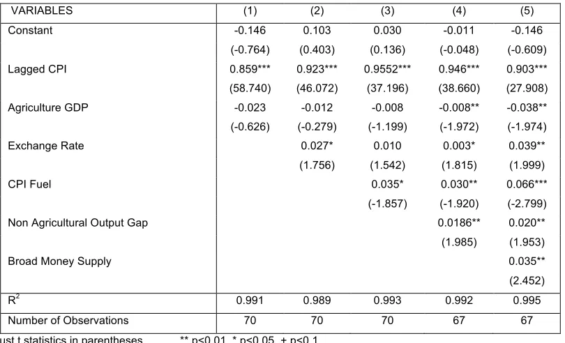
VARIABLES (1) (2) (3) (4) (5) Constant -0.146 0.103 0.030 -0.011 -0.146

(-0.764) (0.403) (0.136) (-0.048) (-0.609) Lagged CPI 0.859*** 0.923*** 0.9552*** 0.946*** 0.903*** (58.740) (46.072) (37.196) (38.660) (27.908) Agriculture GDP -0.023 -0.012 -0.008 -0.008** -0.038** (-0.626) (-0.279) (-1.199) (-1.972) (-1.974) Exchange Rate 0.027* 0.010 0.003* 0.039** (1.756) (1.542) (1.815) (1.999) CPI Fuel 0.035* 0.030** 0.066***

(-1.857) (-1.920) (-2.799) Non Agricultural Output Gap 0.0186** 0.020** (1.985) (1.953)

Broad Money Supply 0.035**

(2.452) R2

0.991 0.989 0.993 0.992 0.995 Number of Observations 70 70 70 67 67 Robust t statistics in parentheses ** p<0.01, * p<0.05, + p<0.1

Source: Database on Indian Economy and Authors’ Calculation

Data on CPI and CPI-Fuel are sourced from Labour Bureau, Government of India, while data on

agriculture GDP and non-agricultural growth rate are obtained from Central Statistical

Organisation. Finally, data on exchange rate and money supply is taken from Database on the

Indian Economy, Reserve Bank of India.

We employ dynamic least squares estimation with lagged dependent variable to identify the key

drivers of inflation. The results are reported in Table (5), where we incrementally add the impact

of the various drivers. Not surprisingly, we find the lagged dependent variable to have a

significant positive impact across all specifications, implying that price rise has been very

persistent in India. Agriculture output negatively impacts inflation, but the effect is not significant

across all specifications. In contrast, exchange rate, defined as the value of foreign currency in

domestic currency has a positive significant impact on prices across most specifications. Thus an

increase in exchange rate, i.e. a depreciation of the domestic currency, raises prices level.

Both fuel prices and broad money supply also exert a positive significant impact on inflation

across the various specifications. Finally, when we introduce non-agricultural output gap as a

proxy for demand side pressures we find that it also have a positive significant impact on CPI

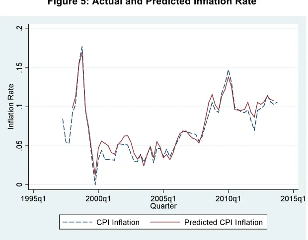
inflation. In Figure 5, when we plot the actual path of CPI inflation with the inflation rate predicted

by the regression specification outlined in Column (5) of Table (5), we find a close match between

Figure 5: Actual and Predicted Inflation Rate

Source: Database on Indian Economy and Authors’ Calculation

On balance, we find that factors, which are traditionally outside the control of monetary policy

such as agriculture output, fuel inflation and exchange rate, do exert a strong impact on

aggregate prices in India. To evaluate the extent of impact of the various variables on prices we

focus on the specification outlined in Column (5) of Table (5). We find that a 1 percent increase

in agriculture output is associated with a 0.39 percent decline in prices, while a 1 percent

depreciation results in 0.4 percent rise in aggregate prices. Fuel prices exert a strong impact on

overall inflation with a 1 percent rise in fuel prices being associated with a 0.68 percent rise in

aggregate prices. In contrast, a 1 percent increase in non-agricultural output growth results in

prices increasing by 0.21 percent. Finally, an increase in money supply leads to prices rising by

0.36 percent. While the above analysis is illustrative and sensitive to the specification chosen, it

nevertheless points to the prominence of factors considered traditionally outside the control of

monetary policy, for inflation in India.

4.3 What should be the appropriate Numerical Inflation Target?

The UPCR recommends a numerical target of 4 percent for CPI inflation with a band of ±2

percent around it. This was driven by both domestic and international factors. On the domestic

front, the UPCR argues that CPI-Combined inflation above 6.2 percent is inimical to growth.

Furthermore, during the period Q4 2003 and Q2 2006, when the output gap was fairly close to

zero, the average CPI inflation was around 4 percent. However, these estimates are sensitive to

period shows that the period 2003Q4 to 2006Q2 was an unusually benign period for overall

inflation, with the various drivers of inflation identified in Table (5), being particularly supportive

during this period to achieve a moderate inflation.

Table 6: Average Values of Key Macroeconomic Variables

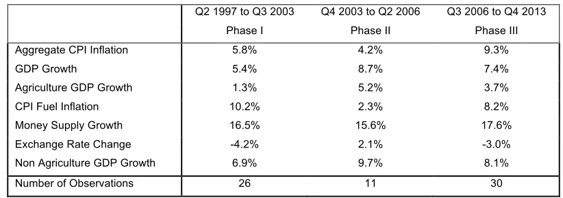
Q2 1997 to Q3 2003 Q4 2003 to Q2 2006 Q3 2006 to Q4 2013 Phase I Phase II Phase III Aggregate CPI Inflation 5.8% 4.2% 9.3%

GDP Growth 5.4% 8.7% 7.4%

Agriculture GDP Growth 1.3% 5.2% 3.7% CPI Fuel Inflation 10.2% 2.3% 8.2% Money Supply Growth 16.5% 15.6% 17.6% Exchange Rate Change -4.2% 2.1% -3.0% Non Agriculture GDP Growth 6.9% 9.7% 8.1% Number of Observations 26 11 30 Source: Database on the Indian Economy and Authors’ Calculations

As evident from Table (6), while agricultural output in Phase II, the period considered in UPCR,

grew at a significantly higher rate than other phases, growth rate of CPI fuel inflation was

significantly lower in Phase II. The domestic currency also strengthened in Phase II on the back

of strong capital inflows, which was in contrast with the other two periods, when there was a

sustained weakening of the Rupee. The growth rate in money supply was also more moderate in

Phase II, despite it recording the highest GDP growth, and help in softening inflation. In contrast,

the demand side pressures were higher in Phase II with non-agriculture GDP growth being the

highest in Phase II.

As pointed out in UPCR and also as documented in Table (6), Phase II was associated with an

average aggregate inflation of around 4 percent. However, there has been a substantial change

in the structure of the economy since then in the aftermath of the Global Financial Crisis

externally, and a host of structural and regulatory bottlenecks stifling growth domestically. Thus, it

becomes pertinent to evaluate the change in aggregate average inflation when the latter period is

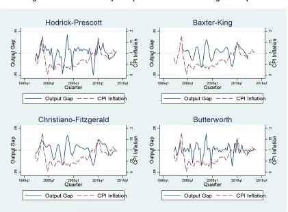
taken into account. Below, we extend the analysis presented in UPCR to 2013Q4. We use four

alternative methods to calculate the gap between actual and potential output growth rate. Apart

from the widely used Hodrick Prescott filter, which removes a smooth trend from a time series, we

also compute the output gap using the Baxter-King filter. The latter is a bandpass filter, which

allows suppression of both the low frequency trend components and the high frequency

components in an economic series. The Christiano-Fitzgerald random walk filter improves over

the Baxter-King filter in terms of an optimality criterion, and do not lose observation. Finally, the

underlying trend of a series. Figure 7 traces the quarterly output gap calculated across the

different filters and the corresponding inflation rates.

Figure 7: Inflation and Output Gap across Different Filtering Techniques

Source: Database on Indian Economy and Authors’ Calculation

Table 7: Average CPI Inflation Rates and Output Gaps

Output Gap of ±2% Output Gap of ±1% Output Gap of ±0.5% Hodrick Prescott 7.8% 7.5% 7.7%

(34) (24) (12)

Baxter King 7.4% 7.1% 7.0%

(29) (19) (8)

Christiano Fitzgerald 7.7% 7.7% 8.0%

(34) (23) (11)

Butterworth 8.0% 7.7% 7.4%

(37) (32) (27)

Note: The numbers in parenthesis denote the number of quarters during which the output gap was within the prescribed range.

Source: Database on Indian Economy and Authors’ Calculation

In Table 7, we report the average inflation rates during the periods when the output gap was

bandwidth of ±2 percent, ±1 percent and ±0.5 percent, and find that the average inflation rate

ranges between 7.1 percent and 8.0 percent across the different filters and bandwidth. Thus,

India’s recent experience shows that periods of small output gap were associated with inflation

rates that were nearly twice than the final target set by the UCPR. Hence, without altering the

structure of the economy by removing the structural and procedural bottlenecks that have stifled

the supply response, reduction of inflation rate to around 4 percent through tightening of

monetary policy, is likely to result in significant deflationary cost. Moreover, an unusually tight

monetary policy could choke off the supply response that is required to alleviate some of the

supply side bottlenecks that have been driving inflation.

The UCPR recommends a glide path for the inflation rate, with the CPI inflation targeted to be

down to 8 percent by January 2015 and 6 percent by January 2016, before formally adopting the

4 percent inflation target with a band of ±2 percent. However, the glide path seems significantly

steep seeking to reduce the inflation rate to almost half its existing level over a period of two

years. This is in sharp contrast to how some of the other developing countries have proceeded in

reaching the final target. For example, in Chile, after nearly a decade in which average inflation

was around 21.5%, the authorities announced in September 1990 the first inflation target range

between 15% to 20%, to be reached by December 1991. The initial goal was to converge to a

single digit inflation, and once that was accomplished, the final goal was to achieve the level of

inflation of developing countries. Thus, from 1991 onwards, each September, the central bank,

announced the inflation target that was to be attained by December of subsequent year. Schmidt

Habel and Tapia (2002) show that the central bank opted for a gradual approach to inflation

stabilization by announcing a new inflation target each year, which was only moderately lower

than the preceding one. Over the decade 1991 to 2001, the annual inflation target was lowered

by 1.5 percent per year. It was only in 1999, when inflation has converged to low stationary levels

and Chile had adopted an exchange rate float, Chile moved to a full-fledged inflation targeting

regime with a range of 2% to 4% and central target value of 3%. The gradualist approach was

adopted considering significant backward indexation of inflation rate in Chile, which would have

caused rapid disinflation to have significant output costs.

Empirical studies estimating the New Keynesian Phillips Curve in India such as Mazumdar (2011)

and Patra and Kapur (2010) find strong evidence for the backward-looking specification, with the

coefficients on lagged inflation being positive and significant. Hence, a rapid disinflation through

monetary tightening to achieve the inflation target in a short period of time is likely to entail heavy

cost.

The extent of fiscal dominance plays an important role in determining the success of an inflation

targeting regime. If the central bank is dominated to the extent that it has to purchase the bonds

issued by the government or lend directly to finance the deficit, then the central bank will be

unable to numerically target an inflation rate. In such a situation the central bank does not have

any control over the size of its own balance sheet, and therefore will be unable to influence the

policy interest rate in response to an excessively high or low inflation rate. In India, the

monetization of fiscal deficits was first reduced and then eliminated in 1997, with government

financing being done increasingly through debt auctions entailing the discovery of risk free

interest rates in the economy. Subsequently, the central bank was prohibited from buying

government securities in the primary market under the Fiscal Responsibility and Budget

Management (FRBM) Act from April 2006.

Blanchard (2004) and Favero and Giavazzi (2004) show that fiscal dominance can also result in

unintended outcomes of monetary policy actions by altering the perception of the financial market

about the ability of the government to honour its external obligations. Consider the case where

the central bank has to raise interest rate in response to a demand shock with inflationary

consequences. If the government’s debt obligations are short-term in nature, there could be

concern in financial markets about debt sustainability which, in turn would widen the risk premium

on the debt. This would likely lead to a weakening of the currency, which would further aggravate

inflationary pressures, in contrast to the original objective of the central bank. Again, India is

relatively well placed on this front as government’s external debt accounts for only 17.9 percent of

the total external debt, and most of this is long term.

Finally, fiscal dominance can have impact on monetary policy through its impact on aggregate

demand and inflationary expectations. With a combined fiscal deficit of around 7 percent of GDP

in 2014-15, fiscal dominance encroaches on monetary policy efficiency, as the central bank has

to undertake open market operations to ‘manage yield’. Furthermore a rise in market borrowing

by the government is associated with crowding out of private investment, which is reflected in a

Figure 8: Fiscal Deficit and Rule Based Targets

Source: Kapur and Mohan (2014) and Authors’ Estimates

Simone and Topalova (2009) argue that India’s experience with fiscal rules has been mixed. India

introduced the FRBM Act in 2003 with the objective of eliminating revenue deficit by 2008-09 and

reducing central government’s fiscal deficit to 3 percent of GDP by 2008-09. However, as shown

in Figure 8, during the period 2004-05 to 2008-09, the actual deficit, including off-budget liabilities

often exceeded the targets set by the FRBM Act as well as those outlined in the 12th Finance Commission. In fact, in 2008-09, official fiscal deficit at 6 percent of GDP was double the target

set under the FRBM Act. Inclusion of off budget liabilities such as oil and fertilizer bonds

amounted to an additional 2.2 percent of GDP in 2008-09.

Part of the deterioration in fiscal deficit can be attributed to various fiscal stimulus measures to

support growth in the aftermath of Global Financial Crisis. However, Simone and Topalova (2009)

estimate these measures to account for only 0.6 percent of GDP. Even in the absence of these

stimulus measures the fiscal deficit would have deteriorated considerably with the introduction of

schemes such as agriculture loan waiver, expansion of National Rural Employment Guarantee

Scheme and implementation of Sixth Pay Commission recommendations, which hiked

government employees’ salaries significantly. The surge in global commodity prices, and absence

of expenditure reforms resulted in subsidies’ bill ballooning dramatically. These measures have

resulted in the actual fiscal deficit breaching the target set by the 13th Finance Commission in recent years with the goal of achieving a fiscal deficit of 3 percent of GDP proving elusive.

Below we estimate the impact of fiscal dominance on inflation following the vector auto regression

(VAR) model outlined in Raj et al (2011). We employ a 4 variable VAR model with the variables

being change in gross fiscal deficit as a percentage of GDP, inflation rate measured as the

change in Wholesale Price Index and the policy rate. The policy rate is proxied by weighted

0% 2% 4% 6% 8% 10%

2003-04 2006-07 2009-10 2012-13 2015-16

F is c a l D e fi c it (% o f G D P)

Fiscal Deficit Off Budget Liabilities

12th Finance Commission 13th Finance Commission

money market rate as it embraces the repo or reverse repo rate depending on the prevailing

liquidity conditions. The final variable is the output gap, which is considered as a proxy for

unemployment rate, as time series data on the latter is not available.

Table 8: Test for Unit Root

Augmented Dickey-Fuller Phillip Perron

Level First Difference Level First Difference Fiscal Deficit -10.164*** -12.593*** -16.204*** -28.083*** Output Gap -4.342*** -8.312*** -4.373** -8.505*** Inflation Rate -2.640* -4.550** -3.027** -4.424** Policy Rate -2.474 -7.229*** -2.459 -7.277*** ***, ** and * indicate significance at 1%, 5% and 10% levels.

Source: Database on Indian Economy and Authors’ Calculation

Prior to conducting the VAR analysis we examine the stationarity properties of the key variables

using the standard Augmented Dicky Fuller and Phillip-Perron tests. The results are highlighted in

Table (8). Apart from the policy rate variable, all other variables are stationary in levels, while all

variables are stationary in first difference.

The optimal lag length of the VAR is selected as one based on various lag length selection

criteria and the ordering of the variables are based on the Granger causality tests. We find that

policy rate being influenced by other variables while fiscal deficit being least influenced. Figure 9

highlights the impulse response functions as a result of a fiscal deficit shock.

A unit positive shock to fiscal deficit immediately increases it and then converges to its long term

equilibrium level after about five quarters. The fiscal stimulus raises the aggregate demand and

has a positive impact on output gap in the next period, and the impact slowly dies down over the

next seven quarters. The impact of the fiscal stimulus to output is evident only in the short run

and could be attributed to the crowding out of private sector investment. An increase in output

gap or an increase in output over its potential leads to a rise in inflation, which takes more than

two years to subside. Finally, we find that monetary policy reacts with a lag and in a cyclical

Figure 9: Impulse Response Function of a Fiscal Deficit Shock

Source: Database on Indian Economy and Authors’ Calculation

The forecast error-variance decomposition shows that shocks to fiscal deficit are important in

explaining the volatility of inflation. These shocks explain about 18 percent of the variation in

inflation after three quarters. Thus it is evident that expansionary fiscal policy by stimulating

aggregate demand leads to a rise in price level in India. Hence, any success of the monetary

policy in containing inflation would be crucially contingent on appropriate fiscal policy.

The UPCR recommends reduction of the central government’s fiscal deficit to 3 percent of GDP

by 2016-17. However, a couple of factors make achieving this target a challenging task. First, the

recently introduced National Food Security Act (2013), aiming to provide subsidized foodgrains to

nearly two-third of the population will entail significant fiscal cost. Gulati et al (2013) estimate the

cost of this Act to be around Rs. 6821 billion over the next three years or an annual average of

1.8 percent of GDP, assuming a nominal GDP growth of 13 percent. Second, additional fiscal

pressures will also arise from the implementation of the recommendations Seventh Pay

Commission, which will revise the salaries of the public sector employees. The implementation of

the recommendations of the Sixth Pay Commission cost the exchequer around 0.7 percent of

5. Conclusion

In this paper we evaluate India’s readiness to move towards an inflation targeting regime. An

estimation of the Taylor Rule for India shows that historically the RBI has put higher emphasis on

inflation rate compared to output gap and exchange rate. This along with RBI gaining greater

monetary independence and allowing more exchange rate flexibility in recent years, places the

central bank in a reasonably good position to initiate a move toward inflation targeting regime.

However, a natural corollary of such a move would be the RBI not stemming volatile movements

of the exchange rate and not being able to shore up reserves. Thus the benefits of lower inflation

need to be balanced with the economic costs associated with exchange rate volatility and low

level of reserves. Other concerns include the efficacy of using CPI inflation as the nominal anchor

given that CPI inflation is much more sensitive to supply side pressures including agriculture

output and fuel prices compared to demand side pressures, and monetary policy has limited

bearing on the supply side drivers. This concern could get accentuated with a conservative

choice of inflation target and band, relative to the structure of the Indian economy, achieving

which might result in significant deflationary cost. Finally, high level of fiscal deficit continues to

remain a strong bottleneck to the success of inflation targeting regime both by stimulating inflation