Discriminative latent variable models for visual recognition

(1)

DISCRIMINATIVE LATENT VARIABLE MODELS

FOR VISUAL RECOGNITION

by

Weilong Yang

B.Eng., Southeast University (China), 2007

M.Sc., Simon Fraser University, 2010

a Thesis submitted in partial fulfillment of the requirements for the degree of

Doctor of Philosophy

in the

School of Computing Science Faculty of Applied Sciences

c

Weilong Yang 2012 SIMON FRASER UNIVERSITY

Fall 2012

However, in accordance with theCopyright Act of Canada, this work may be reproduced without authorization under the conditions for “Fair Dealing.” Therefore, limited reproduction of this work for the purposes of private study,

research, criticism, review and news reporting is likely to be in accordance with the law, particularly if cited appropriately.

(2)

APPROVAL

Name: Weilong Yang

Degree: Doctor of Philosophy

Title of Thesis: Discriminative Latent Variable Models for Visual Recognition

Examining Committee: Dr. Oliver Schulte, Associate Professor Chair

Dr. Greg Mori, Senior Supervisor Associate Professor

Dr. Mohamed Hefeeda, Supervisor Associate Professor

Dr. George Toderici, Supervisor

Senior Software Engineer, Google Research

Dr. Ghassan Hamarneh, SFU Examiner Associate Professor

Dr. Deva Ramanan, External Examiner Associate Professor of Computer Science University of California at Irvine

Date Approved:

ii

(3)

Partial Copyright Licence

(4)

Abstract

Visual Recognition is a central problem in computer vision, and it has numerous potential applications in many different fields, such as robotics, human computer interaction, and entertainment.

In this dissertation, we propose two discriminative latent variable models for handling challenging visual recognition problems. In particular, we use latent variables to capture and model various prior knowledge in the training data. In the first model, we address the problem of recognizing human actions from still images. We jointly consider both poses and actions in a unified framework, and treat human poses as latent variables. The learning of this model follows the framework of latent SVM. Secondly, we propose another latent variable model to address the problem of automated tag learning on YouTube videos. In particular, we address the semantic variations (sub-tags) of the videos which have the same tag. In the model, each video is assumed to be associated with a sub-tag label, and we treat this sub-tag label as latent information. This model is trained using a latent learning framework based on LogitBoost, which jointly considers both the latent sub-tag label and the tag label.

Moreover, we propose a novel discriminative latent learning framework, kernel latent SVM, which combines the benefit of latent SVM and kernel methods. The framework of kernel latent SVM is general enough to be applied in many applications of visual recogni-tion. It is also able to handle complex latent variables with interdependent structures using composite kernels.

(5)

Acknowledgments

I would like to express my gratitude to my senior supervisor, Prof. Greg Mori. I consider myself very lucky to have been his student. I am grateful not only for his constant en-couragement and guidance throughout this research, but also for his patience, kindness and integrity.

Thanks to Prof. Yang Wang for his “unofficial” mentoring. Yang has introduced me to the area of discriminative learning with latent variables, and given me numerous help with my research. Yang is a great mentor, and he is also exceptionally knowledgeable and smart. It is a pleasure to have known him and worked with him.

Thanks to my manager at Google Research, Dr. George Toderici, for giving me the great opportunity to work on “Google-scale”computer vision problems. It was a wonderful experience to work with George and many other world-class engineers at Google.

Thanks to Prof. Mohamed Hefeeda, Prof. Ghassan Hamarneh, Prof. Deva Ramanan, and Prof. Oliver Schulte for serving on my thesis committee and providing constructive suggestions on my research.

Thanks to all my collaborators, labmates, and friends in SFU Vision and Media Lab. Es-pecially thanks to Tian Lan, Guang-Tong Zhou, Arash Vahdat, Peng Peng, Kevin Cannons, and Nataliya Shapovalova for their support and suggestions on my research.

Thanks to the circle of my “Epic Bros”, George Toderici, Annie Toderici, Dat Chu, Sean O’Malley, Tianhong Fang, Yaming Qiu, and Steve Urban, for the encouragement and bless. This thesis is impossible without the many years of support and sacrifice from my family. Lastly, I want to thank my fianc´ee, Yujuan Xie, for her love and support.

(6)

List of Tables

4.1 Results on the still image action dataset. We report both overall and mean per class accuracies due to the class imbalance. . . 46 4.2 Results on the Youtube dataset. We report both overall and mean per class

accuracies due to the class imbalance. . . 46

5.1 Results on the mammal dataset. We show the mean/std of classification accuracies over five rounds of experiments. . . 60 5.2 Results on CIFAR10 Dataset. We show the mean/std of classification

accu-racies over five folds of experiments. Each fold uses a different batch of the training data. . . 62 5.3 Results on object interaction dataset. For the approaches using latent

vari-ables, we show the mean/std of classification accuracies over five folds of experiments. . . 64

6.1 The summary of the sub-tag labels for the 15 tags used in our experiments. Note that our algorithm cannot assign the semantic meaning label to each sub-tag. For the purpose of illustration, we manually assign a word label to each sub-tag by summarizing the video clusters obtained from cowatch initialization. For some sub-tags which are difficult to assign a meaningful word label, we simply use the cluster number to represent them. . . 80 6.2 Precision@1000 for tags “transformers” and “bike”. We compare our method

to the baseline, and a method that runs the first step of our learning procedure once. . . 83

(10)

List of Figures

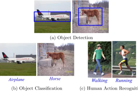
1.1 Examples of visual recognition tasks. The goal of object detection is to local-ize the instances of a particular object in the image, while object classification is only required to predict whether an instance of an object is present in the image. The goal of human action recognition is to identify the actions per-formed by the person in the image or the video. . . 2 1.2 Illustration of different levels of human supervision involved in the training

of a car classifier. . . 3

3.1 Figure (a) is from [86]. Figure (b) and (c) are from PASCAL VOC Challenges [21]. . . 16 3.2 The red bounding boxes illustrate the detection results of a deformable part

model trained for person. The small blue bounding boxes show the latent part locations obtained by inference (Eq. 2.5). This model consists of a root template (a), and a set of part templates (b). (c) visualizes a spatial model for the location of each part relative to the root. These figures are from [26]. 18 3.3 The visualization of latent crop examples. These figures are from [33]. . . 21 3.4 Visualization of an attribute relation graph. An edge on the graph represents

a strong co-occurrence relationship. This figure is from [90]. . . 23 3.5 (a) illustrates the high-level motivation of the model in [91] which is to

rep-resent a human action by a large scale template feature (e.g. optical flow feature) and a set of local “parts”. (b) is the graphical illustration of the model used in [91]. (c) visualizes the latent patches learned during training. Patches are colored based on their part labels. These figures are from [91]. . . 24 3.6 Graphical illustrations of the model used in [45]. The dashed lines indicate

that the structure of latent variables is latent. These figures are from [45]. . . 26

(11)

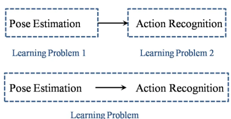
4.1 Illustration of our proposed approach. Our goal is to infer the action label of a still image. We treat the pose of the person in the image as “latent variables” in our system. The “pose” is learned in a way that is directly tied to action classification. . . 32 4.2 Difference between previous work and ours. (Top) Previous work typically

approaches pose estimation and action recognition as two separate problems, and uses the output of the former as the input to the latter. (Bottom) We treat pose estimation and action recognition as an single problem, and learn everything in an integrated framework. . . 34 4.3 Visualization of the poselets for a walking image. Ground-truth skeleton is

overlayed on image. Examples of poselets for each part are shown. . . 36 4.4 Sample images of the still image action dataset [37], and the ground truth

pose annotation. The locations of 14 joints have been annotated on each action image. (a) Running; (b) Walking; (c) Playing Golf; (d) Sitting; (e) Dancing. . . 36 4.5 Examples of poselets for each part from the running action. Each row

corre-sponds to one poselet. The last column is the visualization of the filters for each poselet learned from SVM + HOG. . . 37 4.6 The four part star structured model. We divide the pose into four parts: legs,

left-arm, right-arm, and upper-body. . . 38 4.7 Confusion matrices of the classification results on the still image action dataset:

(a) baseline (b) our approach. Horizontal rows are ground truths, and vertical columns are predictions. . . 45 4.8 Confusion matrix of the classification results of our approach on the Youtube

dataset. Horizontal rows are ground truths, and vertical columns are predic-tions. . . 46 4.9 Example visualizations of the latent poses on test images. For each action,

we manually select some good estimation examples and bad examples. The action for each row (from top) is running, walking, palying golf, sitting and dancing respectively. . . 48

(12)

5.1 Visualization of how the latent variable (i.e. object location) changes during the learning. The red bounding box corresponds to the initial object location. The blue bounding box corresponds to the object location after the learning. 60 5.2 Visualization of some testing examples from the “bird” (a) and “boat” (b)

categories. Each row corresponds to a subcategory. We can see that visually similar images are grouped into the same subcategory. . . 62 5.3 Visualization of how latent variables (i.e. object locations) change during

the learning. The top image is from the “person riding a bicycle” category, and the bottom image is from the “person next to a car” category. Yellow bounding boxes corresponds to the initial object locations. The blue bounding boxes correspond to the object locations after the learning. . . 65

6.1 For the rather specific tag “transformers”, the videos of this tag have large variations in video types and contexts. Those videos can be roughly grouped as video games, two different types of animations, toys, and movies. We use the notation “sub-tags” to refer to those semantic variants and treat them as latent information in our learning framework. . . 68 6.2 The sub-tag initialization results for the “bike” tag. In total, we generate

four sub-tags: “mountain bike”, “falling from bike”, “pocket bike”, and “mo-torbike”. Note that our algorithm only cluster the candidate videos into four clusters and we manually assign a meaningful word label to each cluster. . . 77 6.3 Precision at K curves for both baseline and our method on the 50 million

YouTube video dataset. We incremental increaseK from 100 to 1000. . . 82 6.4 Visualizations of the sub-tag labels of the testing videos for tag

“transform-ers”. . . 84 6.5 Visualizations of the sub-tag labels of the testing videos for tag “bike”. . . . 84

(13)

Chapter 1

Introduction

Recognition is a central problem in computer vision, and its goal is to learn visual categories and then recognize the new instances from those categories. For example, visual recognition seeks the answers to questions such as “Is this a car?” or “What is this object?”. Typical visual recognition tasks include image classification, object detection and classification, hu-man action recognition, etc. Fig. 1.1 illustrates a few examples of visual recognition tasks. A working visual recognition system can have numerous applications in many different fields. For example, face detection has been integrated into many digital cameras to enhance the autofocus. As one of the dominant technologies in biometrics, face recognition has been applied not only in many security systems, but also in the digital photo organizers such as Picasa1 and iPhoto2. The technology of human pose estimation using Kinect sensors [71] is another good example, which achieves a great success in human computer interaction and turns the concept of the controller-free game console into reality. Besides, visual recognition algorithms also play an important role in many image search and video retrieval systems.

The success of visual recognition systems builds on advanced techniques in the machine learning literature, such as AdaBoost, Support Vector Machine (SVM), and Random Forest. Most of these learning approaches for addressing the recognition problems follow the same pipeline which consists of two major steps. First, we need to collect a set of training examples (e.g. images or videos) of given categories. Depending on the details of different applications, each training example needs to be associated with a certain type of label. The second step

1_{http://picasa.google.com}

2_{http://www.apple.com/ilife/iphoto}

(14)

CHAPTER 1. INTRODUCTION 2

(a) Object Detection

Airplane Horse _Walking _Running

(b) Object Classification (c) Human Action Recognition

Figure 1.1: Examples of visual recognition tasks. The goal of object detection is to localize the instances of a particular object in the image, while object classification is only required to predict whether an instance of an object is present in the image. The goal of human action recognition is to identify the actions performed by the person in the image or the video.

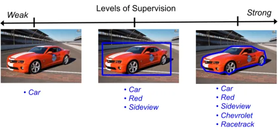
is to learn a model from the training set that can make predictions for the category labels of new examples. The first step of the above pipeline is also known as a process of preparing the training set, which requires manually labeling the training images/videos. For a specific task, e.g. training a car classifier, it may involve different levels of human supervision. For example, as shown in the left image of Fig. 1.2, in a weakly supervised setting, the car image is associated with a category label “car”. This labeling is rather “weak” since it lacks a lot of useful information such as the exact location of the car, the viewpoint (e.g. side-view or front-view), the color or the shape of the car. Whereas “strong” supervision would mark the bounding box or the contour of the car, and even provide a list of descriptive keywords (i.e. attributes) about the image. While the strong labels tend to be more informative and less ambiguous, they are also very expensive to obtain, especially when we have thousands of images. Moreover, developing a system which can combine different types of labeling and maximize the benefits of such strong supervision is also challenging. Therefore, when designing a method for visual recognition, one must consider the trade-offs between the cost of manual labeling and the advantages that it can bring to the learning process.

(15)

CHAPTER 1. INTRODUCTION 3 Levels of Supervision Weak Strong • Car • Car • Red • Sideview • Chevrolet • Racetrack • Car • Red • Sideview

Figure 1.2: Illustration of different levels of human supervision involved in the training of a car classifier.

dataset can be easily collected using keyword search on the Web. However, even after the pruning process by the dataset creators or Amazon Mechanical Turk3_{, there are still} significant intra-category variations and many noisy samples. Typical examples of such datasets are ImageNet [16] and 80 Million TinyImages [78], both of which consist of millions of images and thousands of categories. However, the images are onlyweakly labeled by the category name without further detailed annotations.

In the literature, one possible approach for addressing weakly labeled data is to introduce

latent variables into the training, and treat the missing labels as latent variables. Latent variables refer to the variable that are not directly observed but can be inferred from other observed variables. Latent variables have been widely used in many generative probabilistic models such as latent topic models and hidden Markov models. The constellation model [28] is one of the successful generative models using latent variables for addressing the problem of object classification. However, latent variables are less explored in discriminative models. Note that it is still a debatable topic in the machine learning community whether generative or discriminative models are superior. But in practice, discriminative approaches tend to produce better performance for most recognition problems. There is some recent work which explores the use of latent variables in discriminative models. Quattoni et al. [62] include latent variables in conditional random fields and propose the hidden Conditional

3

(16)

Random Fields (hCRF). Another representative work is the latent SVM which extends the SVM framework for handling latent variables. It is proposed by Felzenszwalb et al. [26] for training a deformable part model (DPM) and achieves excellent performance in object detection.

In this dissertation, we mainly follow the framework of latent SVM, and focus on the learning of discriminative latent variable models for a variety of visual recognition problems. We not only adopt latent variable models for dealing with weakly labeled data, but also generalize them to address the problems ofrecognition with auxiliary labels. In contrast to weakly labeled data, the training data in those problems is associated with certain additional information. For example, in Chapter 4, we consider the task of human action recognition from still images, and each training image is associated with additional human pose labeling. In this case, the main task is human action recognition, and human poses are considered as auxiliary labels.

The major contributions of this dissertation can be briefly summarized as two discrim-inative latent variable models and one general latent learning framework: 1) We propose a latent variable model for the problem of action recognition from still images that jointly learns the actions and poses in a unified framework; 2) We propose thekernel latent SVM

framework which combines the benefits of latent SVM and kernel methods; 3) We propose another latent variable model for addressing the semantic variations of YouTube videos, and we evaluate this model on a very large-scale dataset consisting of over50 million YouTube videos.

1.1 Dissertation Overview

The rest of this dissertation is organized as follows:

Chapter 2 reviews one of the most representative discriminative latent learning frame-works – latent SVM [26]. In the literature, latent SVM has been used to address a variety of challenging problems in visual recognition. The work presented in this dissertation is also mainly based on the latent SVM. In Chapter 2, we first introduce the general formula-tions of latent SVM, then review its two most related models, hidden Conditional Random Fields (hCRF) and MI-SVM in Multiple Instance Learning (MIL).

Chapter 3 reviews a few representative approaches using latent SVM. We mainly cover three sub-fields of visual recognition in this chapter: object detection, object classification,

(17)

and human activity recognition.

Chapter 4 proposes a discriminative latent variable model for addressing the problem of human action recognition from still images. In this model, we treat the pose of the person in the image as latent variables that will help with recognition. Different from other work that learns separate systems for pose estimation and action recognition, then combines them in an ad-hoc fashion, our model is trained in an integrated fashion that jointly considers poses and actions in a unified framework using latent SVM. This work has been published in [95] at IEEE Conference in Computer Vision and Pattern Recognition (CVPR) 2010.

Chapter 5 presents kernel latent SVM – a new learning framework that combines the benefits of latent SVM and kernel methods. We develop an iterative training algorithm to learn the model parameters, and demonstrate the effectiveness of kernel latent SVM using three different applications in visual recognition. Our framework is very general and it can be applied to solve a wide range of applications in computer vision. This work has been accepted to The Neural Information Processing Systems Conference (NIPS) 2012 [96].

Chapter 6 focuses on the problem of content-based automated tag learning on YouTube videos. We propose another latent variable model for addressing the semantic variations (sub-tags) of the videos which have the same tag. In this model, each video is assumed to be associated with a sub-tag label, and we treat this sub-tag label as latent information. This model is trained by a novel latent learning framework based on LogitBoost, which jointly considers both the latent sub-tag label and the tag label. We use cowatch information to initialize the learning process. This work has been published in [94] at IEEE Conference in Computer Vision and Pattern Recognition (CVPR) 2011.

(18)

Chapter 2

Previous Work: Latent SVM

Latent Support Vector Machine (latent SVM) is one of the most representative discrimi-native latent learning frameworks. It inherits the advantages of max-margin learning from SVM, and includes latent variables in the learning process. Due to its elegance and flexibility, latent SVM has been successfully applied to many visual recognition problems, and latent variables are defined in a variety of ways. Before reviewing these applications in Chapter 3, we first introduce the formulation of latent SVM in Section 2.1. We consider structured latent variables and assume there are certain dependencies among the latent variables of a training example. As in other learning algorithms with latent variables, latent SVM is a non-convex problem. We review three commonly used training algorithms of latent SVM in Section 2.2. Lastly, we compare latent SVM with other discriminative latent learning frameworks such as hCRF and MI-SVM in Section 2.3.

2.1 Formulation

We assume a data instance is in the form of (x,h, y), where x is the observed variable and

y is the class label. h is the latent variable that is associated with each instance x. For example, say we want to learn a “car” model from a set of positive images containing cars and a set of negative images without cars. We know there is a car somewhere in a positive image, but we do not know its exact location. In this case,h can be used to represent the unobserved location of the car in the image.

We consider structured latent variables and define h as a vector, i.e. h = (z1, z2, ..), where zi is the i-th component of h and takes its value from a discrete set H of possible

(19)

CHAPTER 2. PREVIOUS WORK: LATENT SVM 7

labels (i.e. zi ∈ H). For structured latent variables, it is assumed that there are certain dependencies between some pairs of (zi, zj). We can use an undirected graph G= (V,E) to capture the structure of latent variables, where a vertexi∈ V corresponds to the label zi, and an edge (i, j) ∈ E corresponds to the dependency between zi and zj. In the original latent SVM work [26], only binary classification is considered, i.e. y ∈ {+1,−1}. Wang and Mori [91] extend latent SVM to multi-class classification. Yu and Joachims [97] further extend it to a more general formulation with structured output. In this chapter, we review the formulation of latent SVM under the multi-class classification setting, i.e. y ∈ Y and Y is a set of discrete class labels. As in other discriminative learning frameworks, we are interested in learning a discriminative function fw : X × Y → R over an instance x and its class labely, where fw is parameterized by w. During testing, we can predict the class label y∗ of an input instance as: y∗ = arg maxy∈Yfw(x, y). The scoring function fw(x, y) is assumed to take the following form:

fw(x, y) = max

h w

>_Φ(_x_,_h_{, y}₎_, _(2.1) where Φ(x,h, y) is a feature vector depending on the instancex, the latent variableh, and the class label y. The maximizing over h in Eq. 2.1 has a very appealing interpretation. For example, in the above “car model” example, the optimalh∗ for the image x(i.e. h∗ = arg maxhw>Φ(x,h, y)) will be the exact location of the car in the image under an ideal situation. One alternative way to define the scoring function fw(x, y) is summing over h instead of maximizing over h. Summing over h corresponds the marginalization rule in probabilistic models. We will compare these two approaches in Section 2.3.2.

Depending on different applications, the model formulationw>Φ(x,h, y) can be defined in different ways. However, in general, given that latent variable h is constrained by an undirected graph G = (V,E), w>Φ(x,h, y) usually consists of unary terms and pairwise terms. Here, we give an example form ofw>Φ(x,h, y) as follows:

w>Φ(x,h, y) =X j∈V w>₁φ1(x, zj, y) + X (i,j)∈E w>₂φ2(zi, zj, y) (2.2) We emphasize that the form ofw>Φ(x,h, y) is not limited to Eq. 2.2. It can be very flexible as long as there exists an efficient inference algorithm for Eq. 2.1.

(20)

2.2 Learning

Given a set ofN training examples{xi, yi}Ni=1, our goal is to learn the model parameter w that can be used to assign the class labely to an unseen instance x. Note again that each training instance is associated with the latent variable hi. Similar to classical SVMs, the optimization in latent SVM is a quadratic program [91] as follows:

min w,ξ 1 2||w|| 2₊_CX i ξi s.t. fw(xi, y)−fw(xi, yi)≤ξi−1, ∀i, ∀y6=yi ξi≥0, ∀i, (2.3)

where{ξi}are the slack variables for handling soft margins, and C is the trade-off param-eter. By replacing fw(x, y) with maxhw>Φ(x,h, y), we obtain the following optimization problem: min w,ξ 1 2||w|| 2₊_CX i ξi s.t. max h w > Φ(xi,h, y)−max h0 w > Φ(xi,h0, yi)≤ξi−∆(y, yi), ∀i, ∀y ξi ≥0, ∀i where, ∆(y, yi) = ( 1 ify6=yi 0 otherwise (2.4)

In the formulation, since the maximum of a set of convex functions is convex, the first component in the constraint (i.e. maxhw>Φ(xi,h, y)) is convex w.r.t. w. However, the second component (i.e. −maxh0w>Φ(x_i,h0, yi)) is concave because of the negative sign. Therefore, the learning problem presented in Eq. 2.4 is a non-convex optimization problem. Unlike other non-convex problems, latent SVM has a nice property ofsemi-convexity. If we fix the latent variableh0 to a single choice for the instance pair of (xi, yi), the optimization problem of Eq. 2.4 becomes convex. In Section 2.2.1 and Section 2.2.2, we will introduce two general approaches of solving the optimization problem of Eq. 2.4. Although neither of these two approaches would guarantee a global minimum or a good local minimum, both of them ensure convergence.

2.2.1 Concave-Convex Procedure

Thesemi-convexity property of the latent SVM allows an intuitive iterative algorithm that alternates between inferring latent variableh0 for the instance of (xi, yi) and optimizing the

(21)

model parameterw. These two major steps are summarized as follows:

1. Holdingw, ξ fixed, compute the optimal latent variable h0 for every instance pair of (xi, yi) :

hi,yi = arg max

h0 w

>

Φ(xi,h0, yi) (2.5) 2. Holdinghi,yi fixed, compute the optimal w, ξ as follows:

min w,ξ 1 2||w|| 2₊_CX i ξi s.t. max h w >_Φ(_x i,h, y)−w>Φ(xi,hi,yi, yi)≤ξi−∆(y, yi), ∀i, ∀y ξi≥0, ∀i (2.6)

Ifh takes its value from a discrete set, Eq. 2.5 can be solved by simply enumerating all possible values of h. However, if latent variables are structured (i.e. h = (z1, z2, ..., zM)), the complexity of this naive enumerating approach isO(MK) when zi takes its value from a discrete set ofKpossible choices (i.e. zi ∈ Hand|H|=K). This is obviously too expensive. Fortunately, in most of approaches using latent SVM, the structured latent variables are assumed to form a tree and then there exist efficient inference algorithms for solving Eq. 2.5, such as dynamic programming.

As we discussed earlier, if holding hi,yi fixed, the optimization problem in Eq. 2.6 is a convex quadratic program. Since it is not in a standard form of multi-class SVMs, we cannot solve it by off-the-shelf SVM solvers (e.g. LibSVM [11] or SVMLight [38]). Wang and Mori [91] develop a solver for Eq. 2.6 based on the cutting-plane method and decomposed dual optimization.

Interestingly, Yu and Joachims [97] show that this iterative algorithm is essentially a concave-convex procedure algorithm. It is shown in [98] that the CCCP algorithm is guar-anteed to decrease the value of the objective function in each iteration and converge to a local minimum. For simplicity, we will refer to this iterative algorithm as CCCP in the following discussion.

2.2.2 Non-Convex Cutting Plane Training

The learning problem in Eq. 2.4 can also be solved by a non-convex cutting plane algorithm in [19], which is an extension of the popular convex cutting plane algorithm [39] for learning

(22)

structural SVM [1]. Due to its ease of use, this algorithm has been adopted in several different applications of latent SVM [95, 90].

First, we write Eq. 2.4 as the following unconstrained formulation:

w∗ = arg min w 1 2||w|| 2₊_CX i Ri(w) where, Ri(w) = max y ∆(y, yi) + max h w >_Φ(_x i,h, y) −max h0 w >_Φ(_x i,h0, yi) (2.7) The learning algorithm in [19] aims to iteratively build an increasingly accurate piecewise quadratic approximation of Eq. 2.4 based on the “sub-gradient”1 ∂w(P_iRi(w)) [19]. The key issue is how to compute the sub-gradient∂w(PiRi(w)). Since

∂w X i Ri(w) ! =X i ∂wRi(w), (2.8)

all we need to do is to figure out how to compute∂wRi(w). We define: (y∗,h∗) = arg max y,h ∆(y, yi) +w T_Φ(_x i,h, y) (2.9) b h0= arg max h0 w T_Φ(_x i,h0, yi) (2.10)

It can be shown that∂wRi(w) can be calculated as

∂wRi(w) = Φ(xi,h∗, y∗)−Φ(xi,hb0, yi) (2.11) The computing of the subgradient ∂wRi(w) involves solving two inference problems in Eq. 2.9 and Eq. 2.10. This is similar to the CCCP learning algorithm (Section 2.2.1) which also requires the solving of inference problems over latent variableh.

2.2.3 Self-paced Learning

The learning of latent SVM is sensitive to initialization and often gets stuck in a bad local optimum. This is a common problem for most non-convex optimization algorithms. In practice, to avoid bad local optima, one needs to run the learning algorithm many times with different initializations, and then choose the model parameters which produce the best performance on a validation set. However, this scheme is computationally expensive.

1

We follow the notation of “sub-gradient” in [19]. It is used to compute the cutting plane which is a “local” lower-bound of the non-convex objective function.

(23)

To addresses these issues, Kumar et al. [42] propose a self-paced learning algorithm for the training of latent SVM. This algorithm is inspired by human learning. For example, children are first taught with simple and easy concepts, and then the hard ones. Similarly, in self-paced learning, training examples are grouped into “easy” examples and “hard” examples. An example is an “easy” one if its correct output can be predicted easily, i.e. it has a higher decision score (above some threshold). Self-paced learning of latent SVM can be considered as a variant of the CCCP learning algorithm in Section 2.2.1. In self-paced learning, the step 2 (Eq. 2.6) is slightly modified and is only performed on the “easy” examples. During the iterations, by adjusting the threshold, more examples will be considered as “easy” and introduced into the training until the entire training set is used. Kumar et al. [42] have demonstrated that this self-paced learning algorithm outperforms the CCCP algorithm on several visual recognition applications. Similar idea has been adopted in [99] which adds training data incrementally at each iteration.

2.3 Related Models

There are many approaches in the literature which are related to the latent SVM. For example, there is a line of work on using latent topic models for visual recognition based on “bag-of-words” representation, such as pLSA [34], LDA [6], etc. The latent topic models are generative and probabilistic so they are very different to the latent SVM. In this section, instead of going through all the learning frameworks with latent variables, we focus on the two most related work to latent SVM: Multiple Instance Learning (MIL) [2] and hidden Conditional Random Fields (hCRF) [62].

2.3.1 Multiple Instance Learning

In the setting of Multiple Instance Learning (MIL), the training examples come in as “bags”. There is at least one example that is positive in a positive bag, while in a negative bag all examples must be negative. It has many applications in visual recognition, such as object detection [84], object tracking [4], etc. Similar to latent SVM, an appealing characteristic of MIL is that the “multiple instance” setting fits with most of visual recognition problems using weakly labeled data. For example, the “car model” example we used in Section 2.1 can also be interpreted as a MIL problem. A positive “car” image is a positive bag which consists of a number of image regions, among which there is at least one region that contains

(24)

a car. Note again that the ground-truth locations of the cars are not provided on the training images. A negative “car” image is a negative bag which does not contain any car region.

A number of researchers have modified classical discriminative learning approaches to perform MIL. Viola et al. [84] propose MILBoost which is an extension of AnyBoost frame-work for MIL problem. Andrews et al. [2] formulate MIL as a max-margin problem and propose the MI-SVM. In MI-SVM, the decision score for a positive bag is defined as the maximum score of the instances in this bag, and the goal of MI-SVM is to maximize the margin between bags instead of instances. The formulation of MI-SVM is defined as follows:

min w,b,ξ 1 2||w|| 2₊_CX I ξI s.t. ∀I, YImax i∈I (w > xi+b)≥1−ξI, ξI ≥0 (2.12) whereYI denotes the label for the I-th bag, andxi denotes the i-th instance in the bag I. Note that this formulation of MI-SVM is for binary classification so thatYI ∈ {+1,−1}. It is interesting to notice that Eq. 2.12 is very similar to the original latent SVM formulation [26]. Indeed, as noted in [26], the latent SVM formulation in [26] is equivalent to the MI-SVM. However, we believe latent variables in latent SVM are much easier to be defined than the “bag-instance” setting in MIL. Moreover, latent variables can be very flexible and have richer representations. For example, in visual recognition, latent variables are often structured (e.g. a tree structure), which are difficult to be formulated in the MIL setting.

2.3.2 hCRF

Quattoni et al. [62] propose the hidden Conditional Random Fields (hCRF) for object recognition. hCRF is a discriminative probabilistic model and it extends the Conditional Random Fields (CRF) model by incorporating hidden variables. Note that the term “hidden variable” in hCRF is equivalent to the “latent variable” in latent SVM. Both of them refer to the variables which are not observed during training. As a discriminative model, hCRF models the conditional distributionp(y|x) directly which can be expressed as follows:

p(y|x;θ) =X h p(y,h|x;θ) = P hexp(Φ(y,h,x;θ)) P y0_,_hexp(Φ(y0,h,x;θ)) (2.13)

whereθare the model parameters, and Φ(y,h,x;θ) is the potential function parameterized byθ. The potential function in hCRF is defined in a similar way to the one in latent SVM,

(25)

and it consists of both unary terms and binary terms if the latent variablehis constrained by a graphE.

The model parametersθ can be learned by minimizing the following objective function, which is equivalent to maximizing the conditional log likelihood:

L(θ) =−X i logp(yi|xi;θ) + ||θ||2 2σ2 (2.14) =−X i logX h exp(Φ(yi,h,xi;θ)) + X i logX y0_,_h exp(Φ(y0,h,xi;θ)) + ||θ||2 2σ2 ,(2.15) where ||_2σθ||22 is the log of the Gaussian prior, i.e. p(θ) v exp(_2σ12||θ||2). The first term in Eq. 2.15 is concave and the other two terms are convex. So, similar to latent SVM, the optimization problem in Eq. 2.15 is not convex. In [62], Quattoni et al. use the gradient descent approach to find its locally optimal solutions.

Both hCRF and latent SVM are discriminative models with latent variables. As noted in [91], we can think of multi-class SVM as a “max-margin” version of hCRF. Wang and Mori discuss the connections between hCRF and latent SVM in [91]. First, the training criteria of latent SVM and hCRF are different. The goal of latent SVM is to maximize the margin but hCRF is to maximize the conditional log likelihood. Besides, the most major difference between these two approaches lies in their different ways of incorporating the latent variables. In hCRF, due to its probabilistic nature, the rule of summing over h is adopted (as shown in Eq. 2.13). In contrast, latent SVM requires the maximizing overh (as shown in Eq. 2.1). It is discussed in [91] that in practice, maximizing over h is more suitable for visual recognition problems. The intuition behind the summing over h (Eq. 2.13) is that the learning algorithm would push the probability of incorrect labeling of h close to zeros and thus the probability of correct labeling of h will contribute more top(y|x;θ). However, this is rather an ideal situation. In practice, for an example x, the choices of its latent variables can be exponentially large, among which only a small number of choices are “correct” ones. Then, the summing overp(y,h|x;θ) may still be dominated by the incorrecth’s, which is obviously not desirable.

2.4 Summary

In this chapter, we have provided an overview of latent SVM. Here, we summarize a few key characteristics of latent SVM as follows:

(26)

• Latent SVM is not convex. A proper initialization is necessary for achieving good performance. Alternatively, one can use some learning tricks, e.g. self-paced learning.

• Latent SVM is essentially a variant formulation of MI-SVM in multiple instance learn-ing (MIL). However, definlearn-ing latent variables for most computer vision problems uslearn-ing weakly labeled data is much more natural than converting them to MIL problems.

• A multi-class latent SVM can be considered as a max-margin version of hCRF. The maximizing over h in latent SVM is more suitable for most visual recognition appli-cations than summing over h.

(27)

Chapter 3

Previous Work: Latent SVM in

Visual Recognition

In this chapter, we review the approaches in the literature which adopt the latent SVM framework for addressing challenging problems in visual recognition. Although these ap-proaches follow the same learning framework, they can be differentiated by 1) the semantic meaning of latent variables; and 2) the model formulation (i.e.w>Φ(x,h, y)). We will focus on these two aspects and review a few representative approaches using latent SVM. We mainly cover three sub-fields of visual recognition: objection detection (Section 3.1), object classification (Section 3.2), and human activity recognition (Section 3.3). We emphasize that latent SVM is not limited to these three applications, and it has been used in a variety of applications, which will be briefly summarized in Section 3.4.

3.1 Object Detection

Object detection is one of the most challenging problems in computer vision. The goal of object detection is to answer the question of “where are the instances of a particular object in the image (if any)?”. Object detection has a wide range of applications in the real world. One successful example is face detection which can be considered as a special case of object detection. Although to a certain extent, face detection is a “solved” problem, the detection of generic objects (e.g. person, car, bicycle, dog, etc.) remains challenging. In this section, we first summarize the challenges of detecting objects. We emphasize that most of these

(28)

CHAPTER 3. PREVIOUS WORK: LATENT SVM IN VISUAL RECOGNITION 16

(a) Shape variations (b) Suboptimal labeling (c) Viewpoint variation

Figure 3.1: Figure (a) is from [86]. Figure (b) and (c) are from PASCAL VOC Challenges [21].

challenges also exist in other applications, such as object classification and human action recognition.

Shape variation: One of the major challenges of object detection is the significant variations in appearance, which include not only illumination and viewpoint variations, but also non-rigid deformations in the shape of the object. For example, people in the pictures are often in very different postures (Fig. 3.1(a)). The linear models (e.g. HOG feature + linear SVM [14]) cannot effectively capture these variations, and they usually only work well when a person is in an upright posture. To handle the variations in the shape of objects, one popular approach is to model the deformable configuration of object parts using pictorial structures [27]. However, it requires the detailed labeling of object parts, which is not available for most object detection tasks.

Suboptimal labeling: In the setting of object detection, images are only manually

labeled with bounding boxes which cover the objects of interest. Although these bounding boxes are treated as “ground-truth”, they are usually suboptimal. For example, as shown in Fig. 3.1(b), the bounding boxes correctly locate the two persons in the image, but clearly the persons in the bounding boxes are not well aligned. It is believed that suboptimal labeling can result in inferior training, and an alignment preprocessing is often necessary. For example, in most face detection/recognition systems, it is a common strategy to first pre-process the face images and align the faces by eye positions.

Viewpoint variations: At present, the general goal of object detection is detecting objects from static 2D images. The projection process of an object from a 3D world to a 2D image plane often results in appearance variations. Compared with the shape variation, the variations caused by the viewpoints or the object poses are much more significant. For

(29)

example, as shown in Fig. 3.1(c), the front-view car looks very different from the side-view car. This type of variation can be easily addressed if we have the annotations of the viewpoints or the objects’ poses in 3D. A successful example is the multi-view face detection system [50] which trains a separate detector for each specified head pose (e.g. frontal face, profile face, etc.). However, for the detection of generic objects, it is difficult to collect accurate annotations of viewpoints or objects’ 3D poses.

So far we have summarized three major challenges of object detection. In fact, all these challenges are not independent from each other and they are rather coupled together. For example, the viewpoint variations would lead to more challenging shape variations or occlusions. Having more complete and elaborate annotations can greatly help us address these challenges, but again it will be difficult and expensive to collect such annotations. In the following sections, we will discuss the literature which adopts the latent SVM to deal with these challenges.

3.1.1 Latent Parts

Felzenszwalb et al. [26] propose a deformable part model (DPM) for object detection. This model achieves the top performance on the PASCAL VOC object detection competition [21] and it has been widely adopted. The DPM builds on the Histogram of Oriented Gradi-ent (HOG) features [14]. Given a set of training images annotated with bounding boxes around each object instance, the training of DPM is a typical binary classification prob-lem. For example, for training a “car” detector, the image regions containing the cars are the positive examples, while other image regions without cars are the negative examples. As we discussed earlier, the bounding boxes provided along with the training set are often not optimal. Therefore, the locations of the optimal bounding boxes are treated as latent variables. Moreover, to address the shape variations, a star-structured pictorial structure model is used in DPM. Unlike other approaches using the pictorial structure, the locations of object parts in DPM are considered as latent, and they will be implicitly inferred during learning.

More formally, the latent variable for an object is defined ash= (z0, z1..., zn), wherez0 denotes the location of the optimal bounding box. (z1, ..., zn) denote the locations of then parts. It is assumed that latent variableh is constrained by a star structure wherez0 is the root. Note that here, for ease of understanding, we modify the notations in [26], and try to make them consistent with the ones in Chapter 2. The potential function w>Φ(x,h, y) is

(30)

Figure 3.2: The red bounding boxes illustrate the detection results of a deformable part model trained for person. The small blue bounding boxes show the latent part locations obtained by inference (Eq. 2.5). This model consists of a root template (a), and a set of part templates (b). (c) visualizes a spatial model for the location of each part relative to the root. These figures are from [26].

defined as follows: w>Φ(x,h, y) =w₀>φ(x, z0) + n X i=1 w>_i φ(x, zi) + n X i=1 diφd(zi, z0) +b, (3.1) whereb is the bias term. φ(x, zi) represents the features extracted from locationzi for the

i-th part. φd(zi, z0) models the relative displacement of the i-th part with respect to the rootz0. The model parametersware simply the concatenation of the parameters in all the factors, i.e. w= (w0, w1, ..., wn, d1, ..., dn, b). The training of DPM is performed by latent SVM and it is solved by the CCCP algorithm described in Section 2.2.1. Because of the star structure, the inference of the latent variableh (Eq. 2.5) can be efficiently computed using dynamic programming and generalized distance transforms (min-convolutions). Example detection results and a part model trained for person detection are visualized in Fig. 3.2.

In DPM, the star structure of latent variables can be considered as a 2-layer structure including a root node and several part nodes. Zhu et al. [99] extend it to a 3-layer structure. In this “deep structure” model, the first layer is the root node (i.e. the optimal bounding box). The second layer consists of 9 child nodes (i.e. parts) in a 3×3 grid layout. Each node in the second layer is associated with 4 child nodes (i.e. parts) from the third layers. They demonstrate the performance of DPM can be improved by simply adding an extra layer in the structure of latent variables. To accelerate the training, an incremental concave-convex procedure (iCCP) is proposed in [99] which adds training data incrementally at each

(31)

iteration and thus reduces the training cost.

3.1.2 Latent Viewpoint

In [26], Felzenswalb et al. use mixture models to address the large viewpoint variations. In their experiments, each mixture model consists of only two components, and each compo-nent corresponds to a viewpoint. Gu and Ren [31] demonstrate that the mixture model representation in DPM is able to handle a large number of components (viewpoints). There is an interesting interpretation of mixture models by latent variables. In [31], each object instance is associated with a viewpoint labelh, where h∈ HandHis the set of all possible viewpoints. Note that different from the structured latent variables we introduced in Chap-ter 2, here the latent variable is a simple discrete value. The potential functionw>Φ(x, h, y) is defined as follows:

w>Φ(x, h, y) =X a∈H

1a(h)·w_a>φ(x, y) (3.2) where 1a(h) is an indicator that takes the value 1 if h = a, and 0 otherwise. φ(x, y) represents the HOG feature extracted from the examplex. Similar to [26], Gu and Ren [31] choose the CCCP algorithm to train the latent SVM models. Note that the latent variable

h in [31] is a discrete value, so the inference of the latent variable is performed by simply enumerating every choice in the set ofH.

In the setting of latent SVM, the viewpoints are considered as latent information. How-ever, in the real world, it might be provided on training data (e.g. 3DObject dataset [66]). Gu and Ren [31] also extend the framework of latent SVM to address the following two sce-narios: 1)h is observed (i.e. ground-truth viewpoint labeling is provided); 2) h is partially observed (i.e. a subset of training examples has ground-truth viewpoint labeling). It demon-strates the flexibility of latent SVM framework for handling the problem of recognizing with auxiliary labels (e.g. viewpoints).

3.2 Object Classification

The goal of object classification is to predict whether an instance of a particular object class exists in the image. It is interesting to notice that if object detection is solved, object classification is solved. For example, if we know there is a car in the right-upper corner

(32)

of the image, then this image definitely contains a car. However, given the challenges we list in Section 3.1, object detection is still a largely unsolved problem, so it is questionable whether the output of any object detection algorithm is reliable enough to be directly used for object classification. Because of the special relationship between detection and

classification, object classification faces the same challenges as object detection. At present, most successful object classification methods are still “global” methods based on the bag-of-features (BOF) extracted from the whole image [21]. This is mainly because the BOF is robust to appearance variations and incorporates scene contextual information.

In this section, we will review two interesting systems for classifying objects with latent variables. We emphasize that the latent variables in these two systems are semantically meaningful. In [33], the locations of objects in the image are considered as latent variables, while in [90] latent variables are the object attributes. It has been experimentally demon-strated that the performance of object classification is improved by using latent variables.

3.2.1 Latent Cropping

As we discussed earlier, most of object classification approaches are “global” approaches based on the bag-of-feature representation and treat each image region equally important. However, consider the bicycle image in Fig. 3.3(a). The bicycle takes only a small portion of the image. Although the “road” in the image may provide a certain amount of contextual information, the “grass” seems irrelevant to the bicycle. Therefore, it is counterintuitive to include all image regions in the training of an object classification model and treat them equally important.

To address this issue, one possible approach is to first localize the most discriminative (or salient) region on the image, then perform object classification on this region instead of the whole image. However, this approach is rather difficult. For example, it is not clear what type of region would be discriminative enough for the purpose of object classification. There is no ground-truth labeling of these discriminative regions either. Instead, Bilen et al. [33] propose to treat the location of the most discriminative region on each image as a latent variable. This latent variable essentially specifies a cropping operation which determines a bounding box covering the most discriminative region on the image. The latent variableh is defined as the location of the discriminative region on the image, and the feature vector Φ(x,h, y) is the BOF extracted from the image regionh. During testing, the inference ofh is performed by enumerating all possible regions on the imagex.

(33)

Figure 3.3: The visualization of latent crop examples. These figures are from [33].

Fig. 3.3 shows examples of the learned latent variables (i.e. the location of the most discriminative region). We can see that all discriminative regions cover the target objects and a bounding box can include more than one object.

3.2.2 Latent Attribute

The goal of object classification is also known as object naming (e.g. “Is this an image of a dog or cat?”). Recently, there is a trend in visual recognition which shifts the goal of recognition from naming to describing. In the task of “object describing”, each image is not only assigned with an object class, but also a list of attributes. Object attributes are in line with human intuition about describing an object. Typical attributes can be color (e.g. “red”), shape (e.g. “round”), materials (e.g. “furry”), etc. There is an interesting question arising: “can attributes help recognition?”. Farhadi et al. [24] propose a two-stage classification process by first training a number of attribute classifiers, then using their outputs to classify objects. They show that the learning of attributes can help categorize objects, especially when only a few training examples are available.

In the two-stage classification framework of [24], the learning of object attributes and classes are treated as two separate learning problems. One limitation of this approach is that the learning of object attributes is not directly tied to the end goal of object classification, and thus the output of the attribute prediction might not be reliable. Wang and Mori [90] introduce a discriminative model which jointly learns object attributes and classes. In particular, they characterize the problem as arecognition problem with auxiliary labels, and treat the attributes as auxiliary labels. The training data consists of both ground-truth object class labels and attribute labels. But testing images do not have the ground-truth attribute labels. The end goal of the learning system is object classification, so the loss functions are only defined over the class labely. This model is trained in the framework of

(34)

latent SVM. To ensure the consistency between training and testing, the auxiliary attribute labels on the training examples are treated as latent variables, so that the learning algorithm would not “overly trust” the attribute information which is missing during testing.

More formally, the attributes of an object are denoted as h = (z1, z2, ..., zK), where

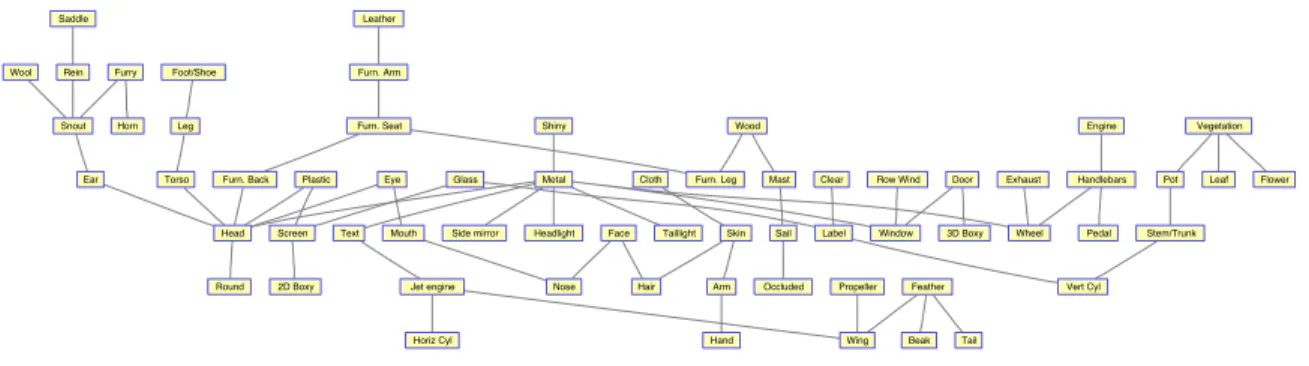
zk∈ {0,1}indicates whether thek-th attribute presents in the image. For example, if thek -th attribute is “red”,zk= 1 means this object is “red”, whilezk= 0 means it is not. Similar to other discriminative frameworks with latent variables, there are certain dependencies (e.g. co-occurrence) between some pairs of attributes (zj, zk), which are captured by an undirected graph G = (V,E). This graph is named as “attribute relation graph”, and an example graph is shown in Fig. 3.4. Thew>Φ(x,h, y) is defined as follows:

w>Φ(x,h, y) =w>_yφ(x) +X j∈V w_zj>ϕ(x) +X j∈V w_y,zj> ω(x) + X (j,k)∈E w>_j,kψ(zj, zk) + X j∈V νy,zj(3.3) Now we briefly describe each potential function in Eq. 3.3. First, w_y>φ(x) is a standard linear model for object classification without considering attributes. Both P

j∈Vw>zjϕ(x) andP

j∈Vw>y,zjω(x) are linear models trained to predict the label (0 or 1) ofj-th attribute for the image x. The only difference is that the latter one is the class-specific attribute model and its parameters wy,zj can be considered as a template for the j-th attribute to take the labelzj if the object class is y. The third potential function P_(j,k)∈Ew>j,kψ(zj, zk) measures the dependencies between thej-th and thek-th attributes, and νy,zj captures the compatibility between object classyand thej-th attributezj. Although this model (Eq. 3.3) is rather complicated, it successfully integrates image featuresx, the latent attribute labels h, and the object class label y in a unified framework which outperforms the two-stage framework in [24].

This paper [90] shares the same motivation as our work that will be presented in Chapter 4, that is to learn a unified framework for the recognition problems with auxiliary labels. In Chapter 4, we address the problem of human action recognition and consider the human poses as the auxiliary labels.

3.3 Human Activity Recognition

Human activity recognition is one of the most popular topics in visual recognition. A lot of work has been done in recognizing human activity either from still images or from video sequences. Much work focuses on recognizing actions performed by a single person. In

(35)

2D Boxy

3D Boxy

Round Vert Cyl

Horiz Cyl Occluded Tail Beak Head Ear Snout Nose Mouth Hair Face Eye Torso Hand Arm Leg Foot/Shoe Wing Propeller Jet engine Window Row Wind Wheel Door Headlight Taillight Side mirror Exhaust Pedal Handlebars Engine Sail Mast Text Label Furn. Leg Furn. Back Furn. Seat Furn. Arm Horn Rein Saddle Leaf Flower Stem/Trunk Pot Screen Skin Metal Plastic Wood Cloth Furry Glass Feather Wool Clear Shiny Vegetation Leather

Figure 3.4: Visualization of an attribute relation graph. An edge on the graph represents a strong co-occurrence relationship. This figure is from [90].

recent years, recognizing and analyzing group activities are increasingly attracting more attention. In general, the goal of human activity recognition is to classify an image or a video sequence into one of several pre-defined categories based on the actions performed by the people in the image or the video. Activity recognition is also a very challenging problem. One of the major challenges is the intra-class variation in action. For example, for the same “walking” action, different people may perform it very differently (e.g. with different strides or speed). A successful human activity recognition system also need to cope with other challenges, such as viewpoint variation, occlusion, and clutter background.

In this section, we will review two approaches addressing human activity recognition using latent variables. One approach [91] focuses on recognizing actions performed by a single person, and the other one [45] focuses on group activity recognition. In both approaches, it is assumed the image frame has been pre-processed so the persons in the image have been localized.

3.3.1 Latent Patch

In visual recognition, the major feature representations include global template, bag-of-words, and part-based models. Inspired by [26], Wang and Mori [91] propose a principled approach to combine the global template features and the part model using latent SVM. The high-level overview of this model is illustrated in Fig. 3.5(a). Different to the pictorial structure model in [26], the part model in [91] is based on the local patches and it models the human action as a flexible constellation of parts conditioned on the appearances of local

(36)

(a)

(b) (c)

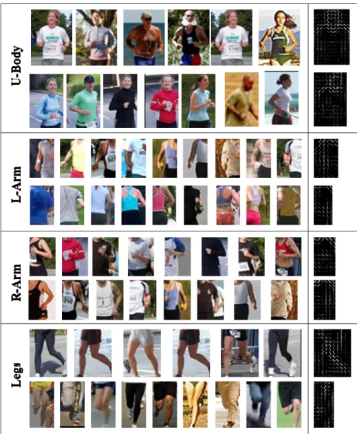
Figure 3.5: (a) illustrates the high-level motivation of the model in [91] which is to represent a human action by a large scale template feature (e.g. optical flow feature) and a set of local “parts”. (b) is the graphical illustration of the model used in [91]. (c) visualizes the latent patches learned during training. Patches are colored based on their part labels. These figures are from [91].

patches. In the model, each local patch is assigned with a “part label” which indicates certain motion patterns of this patch. For example, the patches on the “jumping” person are often assigned with the “part labels” corresponding to the “moving down” or “moving up” patterns. The “part labels” of the patches are treated as latent information.

The training example is assumed to take the form ofx= (s0, s1, ..., sm), wheres0 is the motion feature extracted from the whole frame, si is the feature vector extracted from the

i-th patch. Each example is associated with a vector of latent variables h= (h1, h2, .., hm), wherehidenotes the “part label” of thei-th patch and it takes a discrete value from a setHof possible “part labels”(i.e. hi ∈ H). Again, (h1, h2, .., hm) forms a tree structureG= (V,E),

(37)

which is obtained by running a minimum spanning tree (MST) algorithm over the patches. The model is graphically illustrated in Fig. 3.5. The potential function w>Φ(x,h, y) is defined as follow: w>Φ(x,h, y) =w>₀φ0(y, s0) + X j∈V w>₁φ1(sj, hj) + X j∈V w₂>φx(hj, y) + X (j,k)∈E w>₃φ3(hj, hk, y)(3.4)

w₀>φ0(y, s0) is the root model which models the compatibility of the global feature s0 extracted from the whole frame and the class label y. The second potential function P

j∈Vw1>φ1(sj, hj) captures the compatibility between latent part label hj and the local feature sj on the j-th patch. P_j∈Vw2>φx(hj, y) measures the compatibility of the class labely and the latent part labelhj, and P(j,k)∈Ew>3φ3(hj, hk, y) models the dependencies between part labelshj and hk.

3.3.2 Latent Interaction

Lan et al. [45] focus on recognizing the activities of a group of people. It is believed that the action of an individual in a group is rarely performed in isolation. There are often strong correlations between the actions of the people in the same group. For example, the activity of “queueing” involves a group of people, and the persons in this group usually perform the same action, i.e. standing and facing to the same direction. In [45], Lan et al. propose a discriminative framework using latent SVM, which jointly models the group activity, the individual person actions, and the person-person interactions.

Assuming there are in total m persons found in the image I, the feature extracted from imageI is in the form ofx= (x0, x1, .., xm), wherexi is the feature vector extracted from thei-th person. The collective actions of all the persons in the image are denoted as h = (h1, h2, .., hm), and hi is the action label of the i-th person. Moreover, it is assumed that the persons in the same group are interacted so that there are dependencies between the pair of actions (hj, hk). An undirected graphG= (V,E) is used to capture the structure of the action labels (h1, h2, ..., hm). Fig. 3.6 shows the graphical representation of the model. Comparing Fig. 3.6 with Fig. 3.5, one may notice that the model and notations in [45] are very similar the ones in [91], except that thehin [45] are the action labels of the individuals in the image rather than the part labels. However, there is a significant difference. In [91], h are considered as latent and the graph G (i.e. a tree structure generated by MST) is predefined. But here, the action labelshare assumed to be provided on the training images

(38)

(a) (b)

Figure 3.6: Graphical illustrations of the model used in [45]. The dashed lines indicate that the structure of latent variables is latent. These figures are from [45].

so that they are not latent during training. Instead, the structure (i.e. G) of action labels is treated as a latent variable. This is one of the major contributions of [45]. By treating theG as a latent variable, the person-person interaction becomes adaptive and it achieves better performance than a fixed graph.

Given a set ofN training examples{(xi,hi, y)}N_i=1,the model parameters can be learned by solving the following latent SVM formulation:

min w,ξ≥0,G 1 2||w|| 2₊_CX i ξi s.t. max Gy max h w >_Φ(_x i,h, y;Gy)−max G_yi w >_Φ(_x i,hi, yi;Gyi)≤ξi−∆(y, yi), ∀i, ∀y (3.5)

where w>Φ(xi,hi, yi;Gyi) denotes a potential function in which the action labels hi are constrained by a particular graphG_yi. Lan et al. [45] shows that Eq. 3.5 can be solved using the non-convex cutting plane training algorithm described in Section 2.2.2.

As mentioned earlier, in the setting of [45], the action labels h are observed during training. However, this auxiliary labeling is not provided on the new testing image. This is a very common scenario since the algorithms are usually expected to be fully automatic during testing without using any manual labeling. Therefore, for a new testing image, we need infer both the action labelsh and their structureGy:

fw(x, y) = max Gy max h w >_Φ(_x i,h, y;Gy) (3.6)

(39)

A coordinate ascent style algorithm is proposed in [45] for solving the optimization problem in Eq. 3.6 by alternating between the inference ofh and the inference ofGy.

Lastly, we emphasize that the learning approach in [45] is very different from most of the previous work using latent structured models. It does not predefine any structure for the hidden layer but rather treats it as a latent variable. Again, this learning approach demonstrates the flexibility of the latent SVM framework.

3.4 Other work

In the above three sections, we have reviewed the details of a few interesting approaches which use latent SVM to address the challenging problems in visual recognition. In this section, we will briefly go through other work which follows the same latent SVM framework, but defines different latent variables.

In object detection, to handle the occlusion and truncation on the object instances, Vedaldi and Zisserman [82] assign a binary latent variablehon each HOG cell. For example,

hj = 1 means that thej-th cell of the HOG descriptor is visible, and hj = 0 means this cell is either occluded or truncated. Pandey and Lazebnik [59] directly apply the deformable part models [26] in both scene recognition and weakly supervised object localization. For the weakly supervised object location, it is assumed that the ground-truth bounding-box labeling is not provided on the training set, and it is then treated as the latent variable. A similar part-based model is proposed by Parizi et al. [60]. They represent each scene image as a set of region models (i.e. “parts”), and each image patch is associated with a latent region label.

In human activity recognition, Niebles et al. [54] consider an activity video as a composi-tion of several shorter video segments which represent simpler accomposi-tions. The displacements of these video segments are the latent variables and they are assumed to form a chain structure. Liu et al. [51] introduce the concept of attribute to human action recognition. They use a similar model as [90] and treat the attribute labels as latent variables. Vahdat et al. [81] focus on recognizing the interactions between two persons, and each action is modeled as a sequence of 5 key poses. Both the displacements of key poses in the videos and the choices of key poses (i.e. “which key pose we should use to represent the action at a certain time?”) are treated as latent variables.