On tilt and curvature dependent errors and the calibration of coherence scanning interferometry

On tilt and curvature dependent errors and the

calibration of coherence scanning

interferometry

R

S

,

Y

W

,

J

C

,

R

L

1_{Manufacturing Metrology Team, Faculty of Engineering, University of Nottingham, University Park,}

Nottingham NG7 2RD, UK

2_{Ultra-Precision Optoelectronic Instrument Engineering Centre, Harbin Institute of Technology, 92}

West Da-Zhi Street, Harbin 150001, China

3_{Wolfson School of Mechanical, Electrical and Manufacturing Engineering, Loughborough University,}

Loughborough LE11 3TU, UK

* _{[email protected]}

Abstract: Although coherence scanning interferometry (CSI) is capable of measuring surface topography with sub-nanometre precision, it is well known that the performance of measuring instruments depends strongly on the local tilt and curvature of the sample surface. Based on 3D linear systems theory, however, a recent analysis of fringe generation in CSI provides a method to characterize the performance of surface measuring instruments and offers considerable insight into the origins of these errors. Furthermore, from the measurement of a precision sphere, a process to calibrate and partially correct instruments has been proposed. This paper presents, for the first time, a critical look at the calibration and correction process. Computational techniques are used to investigate the effects of radius error and measurement noise introduced during the calibration process for the measurement of spherical and sinusoidal profiles. Care is taken to illustrate the residual tilt and curvature dependent errors in a manner that will allow users to estimate measurement uncertainty. It is shown that by calibrating the instrument correctly and using appropriate methods to extract phase from the resulting fringes (such as frequency domain analysis), CSI is capable of measuring the topography of surfaces with varying tilt with sub-nanometre accuracy.

Published by The Optical Society under the terms of the Creative Commons Attribution 4.0 License. Further distribution of this work must maintain attribution to the author(s) and the published article’s title, journal citation, and DOI.

OCIS codes: (110.4850) Optical transfer functions; (120.3940) Metrology; (110.0110) Imaging systems; (120.6650) Surface measurements, figure; (120.6660) Surface measurements, roughness; (150.1488) Calibration.

References and links

1. R. K. Leach, Characterisation of Areal Surface Texture (Springer-Verlag, 2013).

2. A. A. G. Bruzzone, H. L. Costa, P. M. Lonardo, and D. A. Lucca, “Advances in engineered surfaces for functional performance,” CIRP Ann. Manuf. Techn. 57(2), 750–769 (2008).

3. H. N. Hansen, K. Carneiro, H. Haitjema, and L. de Chiffre, “Dimensional micro and nano metrology,” CIRP Ann. Manuf. Techn. 55(2), 721–743 (2006).

4. P. de Groot, “Chapter 9. Coherence scanning interferometry,” in Optical Measurement of Surface Topography, R. K. Leach, ed. (Springer, 2011).

5. P. de Groot, “Principles of interference microscopy for the measurement of surface topography,” Adv. Opt. Photonics 7(1), 1–65 (2015).

6. K. G. Larkin, “Efficient nonlinear algorithm for envelope detection in white light interferometry,” J. Opt. Soc. Am. A 13(4), 832–843 (1996).

7. P. de Groot, X. Colonna de Lega, J. Kramer, and M. Turzhitsky, “Determination of fringe order in white-light interference microscopy,” Appl. Opt. 41(22), 4571–4578 (2002).

8. P. de Groot, “The meaning and measure of vertical resolution in surface metrology,” presented at the 5th International Conference on Surface Metrology, Poznan, Poland, 4–7 April 2016.

9. F. Gao, R. K. Leach, J. Petzing, and J. M. Coupland, “Surface measurement errors using commercial scanning white light interferometers,” Meas. Sci. Technol. 19(1), 015303 (2008).

10. P. Lehmann, “Vertical scanning white-light interference microscopy on curved microstructures,” Opt. Lett. 35(11), 1768–1770 (2010).

#278629 https://doi.org/10.1364/OE.25.003297

11. M. Liu, C. F. Cheung, M. Ren, and C. H. Cheng, “Estimation of measurement uncertainty caused by surface gradient for a white light interferometer,” Appl. Opt. 54(29), 8670–8677 (2015).

12. R. K. Leach, “Is one step height enough?” in Proceedings of the 30th Annual Meeting of American Society for Precision Engineering, (Austin, USA, 2015), pp. 110–113.

13. M. R. Foreman, C. L. Giusca, J. M. Coupland, P. Török, and R. K. Leach, “Determination of the transfer function for optical surface topography measuring instruments – a review,” Meas. Sci. Technol. 24(5), 052001 (2013).

14. J. M. Coupland and J. Lobera, “Holography, tomography and 3D microscopy as linear filtering operations,” Meas. Sci. Technol. 19(7), 07010 (2008).

15. J. Coupland, R. Mandal, K. Palodhi, and R. Leach, “Coherence scanning interferometry: linear theory of surface measurement,” Appl. Opt. 52(16), 3662–3670 (2013).

16. M. Born and E. Wolf, Principles of Optics: Electromagnetic Theory of Propagation, Interference and Diffraction of Light, 7th ed. (Cambridge University, 1999), 695–734.

17. W. Xie, P. Lehmann, and J. Niehues, “Lateral resolution and transfer characteristics of vertical scanning white-light interferometers,” Appl. Opt. 51(11), 1795–1803 (2012).

18. P. de Groot and X. C. de Lega, “Interpreting interferometric height measurements using the instrument transfer function,” in Proceedings of the 5th International Workshop on Automatic Processing of Fringe Patterns, W. Osten, ed. (Springer, 2005), pp. 30–37.

19. R. Mandal, J. Coupland, R. Leach, and D. Mansfield, “Coherence scanning interferometry: measurement and correction of three-dimensional transfer and point-spread characteristics,” Appl. Opt. 53(8), 1554–1563 (2014). 20. A. J. Henning, J. M. Huntley, and C. L. Giusca, “Obtaining the Transfer Function of optical instruments using

large calibrated reference objects,” Opt. Express 23(13), 16617–16627 (2015).

21. Zygo NewView 3D optical surface profiler, https://www.zygo.com/?/met/profilers/nexview/.

22. A. J. Henning and C. L. Giusca, “Errors and uncertainty in the topography gained via frequency-domain analysis,” Opt. Express 23(18), 24057–24070 (2015).

1. Introduction

The function and performance of engineered components or micro and nano-manufactured products is highly dependent on their surface topography [1,2]. Traditional contact stylus techniques that provide profiles of surface topography become insufficient for modern manufacturing where simultaneous areal topographic information, fast signal acquisition and nanometre scale height resolution are desired. Optical metrology techniques, such as coherence scanning interferometry (CSI), phase shifting interferometry, focus variation microscopy and confocal microscopy, have been widely employed in the research and manufacturing environment for conducting surface topography measurement and dimensional micro-scale metrology [3].

CSI, also known as scanning white light interferometry, derives information from the interference between light collected from object and reference surfaces when they are both illuminated by the same, broadband source [4,5]. High precision surface height can be calculated from the phase and envelope of the interference signal, for example, using envelope detection methods [6] or the frequency domain analysis (FDA) method [7]. Although CSI commonly achieves a sub-nanometre noise level in surface topography measurement [8], the absolute accuracy is difficult to determine when measuring a surface that is characterized by a wide spectrum in the spatial frequency domain, i.e. the surface contains varying local slope angles and curvatures [9–11]. Traditional step artefacts that contain two parallel flat surfaces are, therefore, not considered sufficient for calibration of CSI systems for measuring complex geometry [12].

object. It should be noted that, in the spatial domain, the object is essentially defined as a 3D distribution (for example density) rather than a two-dimensional (2D) parametric description (for example surface height). This definition is fundamentally different from the traditional characterization of an imaging system, where the field in the object plane is linearly related to that in the image plane by a 2D optical transfer function (OTF) which defines the lateral resolving power [17,18]. The application of a traditional 2D OTF approach to surface metrology is restricted to small surface heights (much smaller than a quarter of wavelength,

λ/4) since only in this regime is the phase of the scattered signal linearly related to the surface height [18]. In the 3D case, however, no such restriction is necessary as the linear characterization is applied directly to the foil model of the surface. In this way, the TF is applied to the spatial frequencies that are inherent in the foil model of the surface.

Under the assumption that the foil model is valid, it has been shown that it is possible to obtain the 3D TF characteristics of a CSI system by measuring the surface of a single sphere [19]. In this preliminary work, the TF of a CSI instrument of numerical aperture (NA) 0.55 was calculated from the interference obtained when measuring a silica microsphere with an estimated diameter of 53 μm. In principle, a sphere of this size provides a convenient calibration artefact as the foil model of this surface contains all of the 3D spatial frequency components that lie within the passband of the instrument and in addition, its radius of curvature means the Kirchhoff approximation can be applied with confidence. Interestingly, Henning et al. pointed out that the foil model of a spherical cap (i.e. portion of a sphere bounded by a circle) contains zeros along its axis of symmetry in the frequency domain and for this reason it was concluded that more than one sphere is necessary to measure the TF [20]. However, this conclusion is incorrect. It is important to realize that the zeros identified were in fact an artefact of the hard cut-off applied to their foil model of the spherical cap and the zeros can be eliminated by applying a degree of apodisation to the edges of the foil model. In addition, it is noted that in the numerical calculation, a foil of finite thickness is required to avoid aliasing problems. In this way, the foil model is in effect blurred such that it is bandlimited, as explained in Section 2.

The 3D TF contains rich information about the metrological characteristics of a CSI system, for example both vertical and lateral resolutions can be derived from the TF and an inverse Fourier transform reveals the point spread function (PSF) [13]. The modulus and phase terms of the TF are usually called the modulation transfer function (MTF) and phase transfer function (PTF), respectively. Once the 3D TF is measured, it is possible to flatten the MTF to enhance the signal response within the passband of the instrument and/or flatten the PTF to compensate for aberration in the imaging system. The combined process will be called “inverse filtering” in this paper, although the effect of flattening the MTF or PTF separately will also be considered. It is clear, however, that errors in the measurement of the 3D TF will lead to errors in the inverse filter, and consequently errors in the surface measurement, and because of this the process must be applied carefully.

In this paper, the calibration and adjustment of a CSI system through the process of measuring the TF and inverse filtering is investigated from first principles. The TF of an ideal (aberration free) CSI system is calculated and fringes are generated for spherical and sinusoidal test surfaces. The MTF flattening afforded by inverse filtering is then explored for the case of surface height measurement from fringes confounded with additive noise. Finally, the introduction of tilt dependent errors through the miscalibration of the ideal CSI instrument is considered. In this case, the TF is measured using a 51 μm radius sphere that is measured/estimated to be a 50 μm radius calibration sphere.

2. Theory

operations. We omit the derivation here but start directly from the linear relationship between the CSI signal and the foil model of the object surface that is defined in terms of the geometry and optical properties of the object. Under the conditions of validity of the foil model, a CSI signal in the 3D spatial frequency domain (k-space) F(k) can be obtained as the multiplication of the TF H(k) and the object function O(k)

( )

( ) ( )

F k = H k ×O k . (1)

O(k) can be calculated from the Fourier transform of o(x,y,z), the object function in the spatial domain, which is defined as [15]

(

)

( )

[

]

o , ,x y z = 4πjRw x y, δ −z s x y( , ) , (2)

where j= −1, R is the Fresnel amplitude reflection coefficient and is assumed to be a complex constant for simplicity if the incident angle is not too large [15], and w(x,y) is a window function with smooth cut-off. The object is defined as an infinitely-thin foil by the 1D Dirac delta function δ(z) based on the surface topography of the object s(x,y). If O(k) is to be obtained numerically by discrete Fourier transform of o(x,y,z), the delta function should be defined as a limit of a Gaussian function

2

2

1

( ) lim exp ,

2 2

z z

σ ε→ πσ σ

− 

δ =  

  (3)

where σ is the standard deviation and ε is a small positive number (ε > 0) that should be chosen to be consistent with the sampling conditions of the discrete Fourier transform calculation. For example, for a system with central wavelength around 0.6 μm and axial sampling distance of 75 nm, σ should not be smaller than 0.14 μm in order to avoid aliasing problems in the calculation.

In the linear theory of surface measurement, the 3D TF of a CSI system can be expressed as [15]

(

)

(

)

( )

2

3

NA 0 NA 0 0 0

H( ) , , d d ,

ˆ

2 G k G k k S ki k

 

 

=_{ } −

⋅

 



k

k k k k

k o (4)

where ki is the illumination wave vector, S(k0) is the spectrum of the source, k0 is the

wavenumber, equal to the reciprocal of the wavelength (1/λ), and GNA(k, k0) is the 3D TF of

an optical system that operates at k0 and is restricted by a finite NA given by [15]

(

)

(

)

(

)

NA 0 2 0 n

0

ˆ

, step 1 ,

4

j

G k k A

k

π

= δ − ⋅ − −

k k k o (5)

where ô is a unit vector in the direction of the optical axis, An is the NA of the system and

step(x) represents a Heaviside step function.

As mentioned earlier, it is possible to measure the TF using a spherical object, as a sphere has a uniformly distributed spatial frequency spectrum. If the CSI fringe data of an object in the spatial domain, f(x,y,z), is acquired, and the geometrical dimensions of the sphere are known, then the TF can be calculated as

( )

( )

_{( )}

H = ,

O k k

k (6)

of a CSI system, which can be calculated using Eq. (4). The low and negative frequency components in the kz direction and high frequency components in kx and ky directions of the

TF are filtered as they do not contribute to the interference signal.

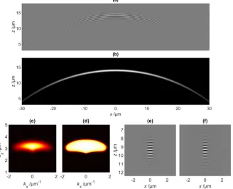
The calibration process is shown in Fig. 1 for a system with 0.55 NA, central wavelength

λ0 = 0.58 μm, and full width at half maximum (FWHM) bandwidth Δλ = 0.08 μm. The phase

term of the TF is not shown as it has a constant value (zero) over the entire spectrum as a consequence of the absence of aberration in the ideal system considered in this paper.

Fig. 1. Calibration of the 3D TF of a CSI system by measuring a spherical object. Cross-sectional views of a) the CSI fringe data (0.55 NA, λ0 = 0.58 μm and Δλ = 0.08 μm); b) foil model of the surface (sphere radius of 50 µm); c) normalised MTF (note the phase term is zero); d) flattened MTF; e) original PSF and f) filtered PSF.

It is noted that the Fourier transform of H(k) gives the PSF of the CSI (see Fig. 1(e)). Alternatively, given the source spectrum, the NA of the CSI system and the surface topography of the object, the CSI fringe data can be simulated using Eq. (1) - Eq. (5).

A gain function g(k) can be calculated based on the measured MTF to enhance and flatten the MTF (see [19] for details of this procedure). The flattened MTF is shown in Fig. 1(d), and the resulting change of the shape of the PSF is shown in Fig. 1(f). Flattening of the PTF is done by multiplying exp[−jθ(k)] with H(k), where θ(k) is the phase of H(k) and should be zero in the ideal CSI system, unless the calibration procedure is not carried out correctly, for example in the presence of radius error of the calibration sphere, as discussed later.

In this paper, 2D cross-sectional views through planes y = 0 or ky = 0 of the CSI fringe

data, the surface topography and the TF will always be used for display purposes as the 3D TF of an ideal CSI system is symmetrical about the kz axis (parallel to the direction of the

3. Methodology

The general assumptions and conditions of this study are: 1) The surfaces of the simulated objects meet the Kirchhoff approximation, i.e. the surfaces are slowly varying on the optical scale; 2) The surface geometry is such that the effects of multiple scattering can be neglected; 3) The simulated CSI system is aberration-free, such that the PTF of the simulated CSI system is zero (note that we will address the effects of defocus and aberration in a subsequent paper); 4) In order to minimize the impact of the algorithm that calculates the surface height from the CSI fringe data, the a priori height information of the nominal surface is used to find the phase of the fringes at the surface. It is then assumed this phase is linearly related to an error in the surface height by the factor 2π/λ0. In the following, we will refer to this as direct

phase analysis. By way of comparison, we have also implemented the FDA method [7]. The FDA algorithm finds the phase of the most significant peak within the 1D Fourier transform of the column-wise fringe data in the axial direction.

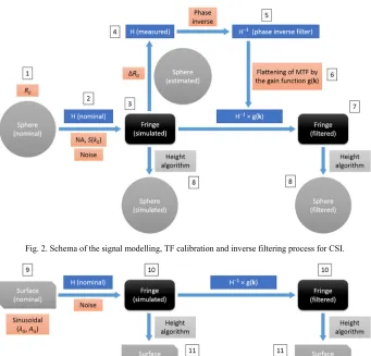
The methodology of this study is illustrated in the flow charts in Fig. 2 and Fig. 3, in order to help the readers to understand the concept and implementation of the calibration approach using spherical objects.

1. The foil model, o(x,y,z) of a nominal spherical cap is created of which the radius R0 is

known. This sphere does not exist in reality as it is impossible to obtain a perfect sphere and the true value of its radius by any measurement. This is a key advantage of doing a simulation study. The object function is calculated based on Eq. (2). 2. Given the NA, source spectrum (usually a Gaussian distribution is assumed) and noise

level of the CSI system, the nominal TF can be simulated based on Eqs. (4) and (5). 3. Given the Fourier transform of the object function, F(k) is calculated from Eq. (1) and

the fringe data f(x,y,z) can be calculated by the inverse Fourier transform of F(k). The simulated fringe data is effectively equivalent to that which can be obtained from a single experimental CSI measurement.

4. Starting from the simulated fringe data, we can now measure the TF based on Eq. (6), by introducing a calibration sphere of radius RC, which can only be estimated from

reference measurements. The difference between the measured and nominal radius

ΔR0 = RC−R0 is the key variable in this study.

5. Obtaining the PTF. If the radius of the calibration sphere is incorrect, i.e. ΔR0 ≠ 0,

some variations in the measured PTF will occur. The effect of this error provides one of the major motivations of this study.

6. Flattening of the measured MTF by the gain function g(k) (see Fig. 1(d)). This procedure may enhance the visibility/contrast of the original fringe, particularly in the regions with high surface slopes. However, the system noise, if present, will also be amplified and the signal-to-noise ratio (SNR) will drop.

7. Applying the inverse filter (with flattened MTF and PTF) to obtain a filtered set of interference fringes.

8. The surface height is calculated from the fringe data using the direct phase and FDA algorithms. At this stage, we have three spheres – the nominal sphere, the simulated and the inverse filtered sphere. The simulated and inverse filtered CSI results can be compared with the nominal value directly to obtain the deterministic difference of surface height.

10. Similar to step 3, the fringe data of the surface can be simulated using the nominal TF. By applying the previously obtained inverse filters, the fringe data is modified. 11. Similar to step 8, the surface height of the simulated and inverse filtered surfaces can

be calculated and compared with the nominal values.

Fig. 2. Schema of the signal modelling, TF calibration and inverse filtering process for CSI.

Fig. 3. Schema of the signal modelling and inverse filtering of CSI measurement of surfaces.

Clearly, the absolute deterministic difference between the nominal and the CSI measured surface topography can only be obtained in a simulation study. In addition, it is much easier to qualitatively and quantitatively understand the effects of the large number of parameters that impact the CSI signal formation through simulations, rather than a limited number of experiments.

4. Results and discussion

4.1 Verification of CSI signal modelling

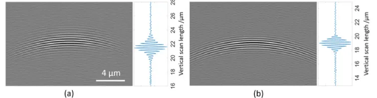
With the parameters An = 0.55, λ0 = 0.58 μm and Δλ = 0.08 μm (based on the configurations

of Zygo NewView 5000 [21] which was used in the experiment), the fringe data is simulated for a silica sphere with radius of 21.5 μm. Zero-mean Gaussian white noise is added to the simulated fringes to mimic the image noise in the CSI system. The FWHM bandwidth of the simulated source spectrum is slightly different from that of the experimental system because the experimental spectrum is not an ideal Gaussian. Unless otherwise stated, these parameters will be used throughout the following simulations. As shown in Fig. 4, a good qualitative agreement is achieved between the simulation and experiment.

Fig. 4. Cross-sectional CSI signal of the calibration sphere (R0 = 21.5 μm) and the signal

profile through the top of the sphere, of the experiment (a) and simulation (b).

4.2 Errors in CSI, and the effects of inverse filtering and noise

Under the assumption that there is no noise in the system, the fringes generated by a sphere with 50 μm radius are simulated using the ideal 3D TF of a CSI system that is calculated from Eq. (4). Assuming R0 = RC = 50 μm, the correction of the TF can be accomplished using the

inverse filtering operations discussed previously. The expected height error of the CSI measurement of the nominal sphere is revealed by subtracting the height profile of the nominal sphere from the height measurements obtained from the simulated or filtered sphere as shown in Figs. 5(b) and 5(c). The surface heights are calculated from the simulated and inverse filtered fringe data by the direct phase and FDA algorithms.

The result shows that an ideal (aberration-free) CSI system can be expected to measure a sphere with height error of a few nanometres within the maximum detectable area. Both the direct phase and FDA algorithms generate very similar results within the area |x| < 25 μm, corresponding to a surface slope of 30°. It is noted that the error observed close to the edge of the maximum detectable region corresponds to low contrast fringes and can be easily cut off by applying a threshold in the algorithms. It is also noted that the errors observed with both the FDA and direct phase methods are significantly less than the errors reported by Henning et. al. under similar conditions [22]. We have found, however, that the implementation of the FDA method is critical, for example the number of points in the fast Fourier transform should be a power of two and match the number of sampling points of the fringe.

The red dashed curves in Fig. 5 show the result of the inverse filtered CSI measurements of the sphere with flattened MTF. Both algorithms improve the height error for |x| < 20 μm, corresponding to a surface tilt of around 24°, but the error increases rapidly at the edge of the spherical cap where the surface tilt is greatest. This is probably because the modified PSF contains oscillating and strong side lobes as shown in Fig. 1(f). It is noted that the inverse filter without a flattened PTF has no impact on the surface height measurement because when the radius error ΔR0 = 0, the PTF is identically zero for an ideal CSI system. The effect of ΔR0

Fig. 5. Surface height profiles (a) of the calibration sphere (R0 = 50 μm and ΔR0 = 0, profiles

offset by 10 μm for display purpose; black curve shows the nominal surface), and height error of the simulated (solid blue) and the inverse filtered (dashed red) sphere calculated using the direct phase method (b) and FDA method (c).

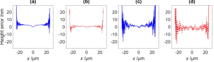
Because the flattened MTF effectively boosts certain regions of the TF through the gain function, the decrease in measurement error shown in Fig. 5 is expected to be accompanied by an increased sensitivity to noise. Noise in a CSI measurement is caused by a combination of many factors, such as the detector noise and environmental disturbances. The effect of additive white noise on the measurement of a sphere is shown in Figs. 6(a) and 6(c). A tilt dependent random error in the CSI measurement, similar to the effect that was reported in an experimental study of surface roughness measurements [11], is observed. The error is attributed to the fact that the MTF drops at high spatial frequencies in the kx direction, that

corresponds to large surface tilt (see Fig. 1(c)), while the white noise is uniformly distributed within the passband such that the SNR decreases. In the presence of noise, the gain function should be used with caution. Figures 6(b) and 6(d) show that the inverse filtering can make the measurement significantly worse if the noise increases from 1% to 4% (root-mean-square (RMS) value).

Fig. 6. Effect of noise on CSI measurement of a sphere (R0 = 50 μm and the TF is correctly

calibrated as ΔR0 = 0); The height errors of the simulated (a) and inverse filtered (b) spheres

with 1% RMS noise relative to the fringe modulation peak, and the height errors of the simulated (c) and inverse filtered (d) spheres with 4% noise. The direct phase algorithm is used.

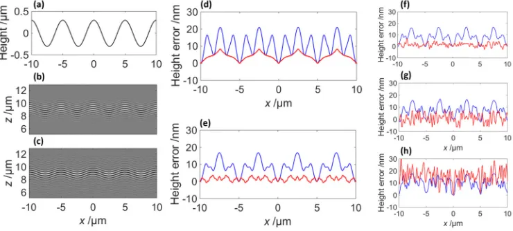
We can now study CSI measurements of other surfaces and the effects of the obtained inverse filter (with and without noise). Sinusoidal surfaces are used as a reference for this task because they are single frequency and because non-linear behavior is evident through the generation of higher harmonics. The surface profile, the simulated and inverse filtered fringes and the corresponding height errors for a sinusoidal grating surface with period λG = 5 μm and

amplitude AG = 0.3 μm are shown in Fig. 7. The surface topography is shown in Fig. 7(a)

in Figs. 7(d) to 7(h). Figures 7(d) and 7(e) show the height errors obtained by the direct phase and FDA algorithms, respectively. The latter performs slightly better than the former, and the flattening of the MTF by the inverse filter reduces the errors to the nanometre level.

It is also evident that although the errors are associated with, they are not exclusively due to, surface tilt. If this was the case, we would expect the height error to be zero at both the peaks and troughs of the sine profile. However, the error is also strongly dependent on the local curvature of the surface, and the inverse filter with flattened MTF may effectively reduce this curvature dependent error. Furthermore, the errors exhibit higher harmonics and this characteristic shows that the measurement process as a whole is becomingly increasingly non-linear.

The effect of the flattening of MTF in the presence of 1%, 2% and 4% RMS additive noise is shown in Figs. 7(f) to 7(h), respectively. It can be seen that in this case that the improvement due to the flattened MTF is negated by the additional noise sensitivity at around 4% RMS.

Fig. 7. CSI measurement of a sinusoidal surface with λG = 5 μm and AG = 0.3 μm; a)

cross-sectional surface profiles; b) the simulated CSI fringes; c) the inverse filtered fringes; d) the height errors calculated from the simulated (solid blue) and filtered fringes (solid red) by the direct phase algorithm; e) the height errors calculated from the simulated (solid blue) and inverse filtered fringes (solid red) by the FDA algorithm; f), g) and h) show the height errors calculated by the FDA algorithm for the fringes with noise levels of 1%, 2% and 4%, respectively.

4.3 Effects of radius error of calibration sphere

Fig. 8. Schema of geometrical errors of a sphere: a) asymmetrical error; b) symmetrical error; c) radius error.

However, the measurement of sphere radius remains a highly challenging metrology problem if accuracy is required at the nanometre level. Therefore, the effects of the radius error of the calibration sphere needs to be studied.

It is interesting to consider the effect of correcting the TF of an ideal CSI system based on the measurement of a calibration sphere of unknown radius. Using the CSI system parameters mentioned previously, and letting R0 = 50 μm and ΔR0 = 1 μm, the measured TF is shown in

Fig. 9. While the MTF is essentially identical to that of Fig. 1(c), the change in the PTF is pronounced, as the phase value should be zero within the system bandwidth. The phase distortion is especially strong in the high spatial frequency regions along the kx axis, and will

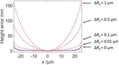
be propagated to the corresponding inverse filter. When the phase inverse filter is calculated in this way, the resulting phase error is essentially the surface height error at a given tilt angle. This is shown in Fig. 10. Here the measurement error is plotted as a function of position together with the height difference between the nominal and real calibration spheres for a range of ΔR0. If 1 nm additional tilt dependent error is desired within 30° surface tilt, the

radius error of the calibration sphere should be smaller than 6 nm.

Fig. 9. The normalised magnitude (a) and the phase (b) of the measured TF with the radius error ΔR0 = 1 μm.

Fig. 10. Height error of CSI measurement of a sphere (R0 = 50 μm) after the phase inverse

filtering (without the gain function) based on the correct (solid blue) and incorrect (dashed red) calibrations of the TF for ΔR0 = 0.01 μm, 0.1 μm, 0.5 μm and 1 μm, respectively. The FDA

algorithm is used.

The additional surface height error due to the miscalibration as a function of ΔR0 and the

but it is also found that R0 does not affect the result because the TF of a system is not

determined by the calibration object, and the NA of 0.3 and 0.4 will generate very similar tilt dependent height errors within their maximum detectable tilt angles, approximately 17° and 23°, respectively. By using this figure as a lookup table, the readers may estimate the surface heights errors for their own samples.

Fig. 11. Additional height error as a function of ΔR0 and the surface slope angle.

It is also interesting to consider the effect of measuring sinusoidal samples with a CSI system that has been calibrated using the same wrong-sized reference sphere (R0 = 50 μm and

radius error ΔR0 = 1 μm). The profiles and the height measurement errors of the three

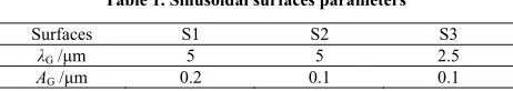
surfaces, S1 to S3 defined by the parameters in Table 1 are shown in Fig. 12.

Table 1. Sinusoidal surfaces parameters

Surfaces S1 S2 S3

λG /μm 5 5 2.5

AG /μm 0.2 0.1 0.1

In Fig. 12, the red and blue curves show the height errors of the filtered surfaces with and without the radius error of the calibration sphere, respectively; the dashed and solid curves show the inverse filtering with and without the flattening of the MTF, respectively. The measured surfaces are aligned by their peak positions as we assume there are no height errors of the CSI measurements of the peaks, as they are locally flat. Therefore, the height errors are always zero at x = 0. The phase inverse filtered surfaces (solid blue curves) should be exactly the same as the original measured surfaces in the absence of noise and aberration. It is observed that:

1) Pronounced tilt dependent errors are noticed for the case of the miscalibrated instrument (see Fig. 12(a)). The errors are on similar levels for S1 and S3 which have similar maximum surface slopes. It is noted that because the error is proportional to the magnitude of the surface tilt (see Fig. 10), miscalibration results in a periodic function with a strong component at twice the surface frequency. 2) Because the error is a non-linear function of surface tilt (see Fig. 10), the error is

reduced significantly as the amplitude of the sinusoidal surface topography is reduced (see Fig. 12(b)).

3) Flattening of the MTF reduces the tilt and curvature dependent errors as the dashed curves are always lower than the solid curves.

4) The tilt dependent errors are positive valued as ΔR0 = 1 μm, and the errors are negative

Fig. 12. Profiles (upper) of CSI measurements of sinusoidal grating surfaces a) S1, b) S2 and c) S3, and the corresponding height errors (lower) after the inverse filtering. The red and blue curves show the height errors of the filtered surfaces with and without the radius error of the calibration sphere, respectively; the dashed and solid curves show the inverse filtering with and without the flattening of the MTF, respectively. The FDA algorithm is used.

5. Conclusions

In this paper, a recent proposed method [19], based on the foil model of the surface [15], for the calibration and adjustment of the 3D TF of a CSI system has been investigated. The accuracy of the calibration method relies on the accuracy of the geometrical dimension of the calibration sphere. The effects of the radius error of the sphere and the measurement noise introduced during calibration and adjustment of the 3D TF of CSI are investigated. This knowledge, which is currently missing in the literature, is essential for determination of the feasibility of this calibration method for CSI systems.

In general, it is possible to calibrate a CSI system with a single sphere. When implementing this method in a digital environment, care must be taken to ensure that additional errors are not introduced by the process of aliasing.

If optical aberration exists in a CSI system, distortion in the PTF can be expected. The phase distortion can be measured using a calibration sphere and corrected by applying the phase inverse filter. However, the radius error of the calibration sphere results in errors in the measured PTF, and the errors cause tilt dependent errors in the surface height measurement when the phase inverse filter is applied. An ideal (aberration-free) CSI system is simulated in this paper because the phase error can be observed directly. If 1 nm additional height error (due to the incorrect calibration) is desired at 30° surface tilt, the radius error of the calibration sphere should be smaller than 6 nm. In this paper, the additional height error as a function of the radius error and the surface slope angle is provided for the readers to estimate the additional inverse filtering error for their own surfaces.

It has also been shown that, in the absence of noise, the performance of a CSI system can be further improved by using a gain function to flatten the MTF of the instrument, especially the curvature dependent error can be reduced effectively. It has been noted, however, that in the examples tested that the advantages of this approach are negated if the RMS noise levels exceed approximately 4% and the random error due to high noise level may dominate the systematic error. It has also been found that the random error is tilt dependent as a result of the reduced SNR in high spatial frequency regions in the kx direction.

In summary, this work provides further evidence to support the capability of calibration and adjustment of CSI instruments using spherical calibration artefacts and inverse filtering methods. The method may also be appropriate for the calibration and adjustment of other 3D optical imaging techniques, such as confocal microscopy and optical coherence tomography.

Funding

Engineering and Physical Sciences Research Council (EPSRC) (EP/M008983/1).

Acknowledgment