Automated mesh generation for the rotator section of a radial inflow turbine

(1)

University of Twente

Internship report

Automated mesh generation for the

rotator section of a radial inflow turbine

Author:

Tjarke van Jindelt

Supervisors:

Dr. Peter Jacobs

(2)

(3)

List of Figures

1.1 Sketch of a radial inflow turbine

. . . .

2

2.1 Unstructured and structured grids

. . . .

4

2.2 Grid topologies

. . . .

4

2.3 Example of Mapping

. . . .

5

2.4 Sketch of the computational domain

. . . .

6

2.5 Rotator topography

. . . .

6

3.1 Display of the input camberlines

. . . .

8

3.2 Surface sketch

. . . .

9

3.3 Structure of the computational domain

. . . 10

3.4 Photo of a rotator section of a radial inflow turbine

. . . 11

3.5 Display of the computational domain

. . . 11

3.6 Display of the complete topology

. . . 12

A.1 Arrangement of a hexaedral block in Eilmer3

. . . 16

A.2 Structure of the computational domain

. . . 17

(6)

(7)

Chapter 1

Introduction

World wide energy consumption is increasing, which is a challenge that is facing many

societies. Paired with ecological threats such as climate change and smog the need for

more renewable energy is apparent.

A contribution can be made with geothermal energy. Australia has enough geothermal

energy to provide the countries electrical energy needs for 450 years according to an

es-timate by the Centre for International Economics[

1 ]. Though many technical challenges

still have to be solved to be able to extract this energy.

Another provider could be solar energy. Which can be obtained on a large scale in

Australia’s Deserts, as well as on a smaller scale locally.

Both solar and geothermal energy can be converted to electrical energy using turbines

driven with fluids heated by either source of energy. Here the optimal shape depends

on different parameters such as type of fluid, temperature of fluid, flow rate, etc. These

parameters can change per site and application. Therefore an automated approach to

design and optimize turbines is needed.

This internship builds on work done by C.A. de Miranda Ventura on radial inflow

tur-bines for renewable power generation applications [

2 ]. A sketch of a radial inflow turbine

is given in figure

1.1 .

(8)

Chapter 1. Introduction

2 Flow

Stator

Rotor

_Hub

Shroud

Rotor

Stator

Flow

pressure side

suction side

[image:8.596.94.468.82.309.2]

Rotational axis

Figure 1.1:

Sketches of a radial inflow turbine from different perspectives (after [

2 ])

1.1 Objective and scope of the internship

The objective of this internship is to create an automated grid generation tool for one

blade section of the rotator of a radial inflow turbine. The input provided are curves

describing the blade at various hub to shroud locations.

This can then be used in a larger project to create a automated process of examining,

(9)

Chapter 2

Background on meshes

2.1 Introduction

In Computational Fluid Dynamics (CFD) the flow is generally simulated with a finite

volume approach. Which means the area one is interested in is separated into many

small volumes. For each of these smaller volumes the flow quantities are determined

through fluxes over their surfaces.

This conglomerate of volumes is called a mesh and the size and shape of its volumes

determine whether or not a flow solver is able to accurately compute the flow one is

interested in.

While smaller control volumes may be able to resolve even smallest scales of turbulence

they also result in a larger amount of volumes per mesh.

The amount of volumes

determines the time that is needed to compute the flow.

This time can mount up

to unreasonable durations quite easily when fine meshes for practical applications are

considered, especially when just a quick estimate is needed.

In this chapter a short explanation of meshing approaches is given and after that the

mesh topology that will be used for the radial inflow turbine is explained.

2.2 Structured and unstructured meshes

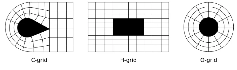
There is a distinction between structured and unstructured grids of which examples are

shown in figure

2.1 .

The unstructured grid offers more flexibility in its creation, as the nodes (corners of

a volume element) can be placed more freely. Therefore, unstructured grids have less

problems when dealing with complex geometries and usually contain less nodes.

(10)

Chapter 2. Background on meshes

4 In contrast the clear order of blocks in the structured grid prescribes certain node

dis-tributions. While the structure normally increases the number of grid points, it also

leaves some opportunities to save memory during calculation. This then allows different

solving methods and can cut solving time.

Besides, there are flow features that are resolved better when structured grids are used

e.g. boundary layers and vortices.

Eilmer3 is a flow solver that uses structured grids and therefore the grid that is created

will be structured, where hexahedral elements are used.

[image:10.596.101.463.256.380.2]

Unstructered grid

Structured grid

Another structured grid

Figure 2.1:

Examples of unstructured and structured grids

2.2.1 Topologies

There are different ways to structure a grid. The overall order is called the topology

and three examples are given in

2.2 . Here, the mesh is created around the black object

in the center of each grid. The nomenclature of these topologies is straight forward, as

they resemble letters of the alphabet.

In a grid highly skewed elements should be avoided. Therefore, round objects can be

meshed best with an O-grid type approach, while square corners can be discretised with

an H-grid approach.

C-grid

H-grid

O-grid

[image:10.596.87.473.613.728.2]

(11)

Chapter 2. Background on meshes

5

2.2.2 Mapping

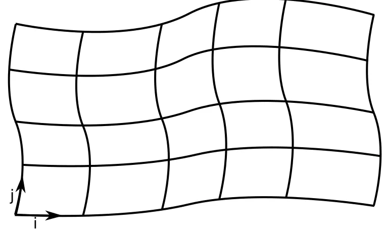
As said before, the structure of the mesh allows for different solving methods. This

includes mapping from physical to computational coordinates. An example is shown in

figure

2.3 , where i and j are the computational coordinates.

Ordering mesh elements according to their computational coordinates can be done

straight forward. This way the interfaces between elements can be identified more easily

and reduce computational effort.

Mapping is used in the next chapter to create lofted surfaces, too.

i

j

i

y

x

[image:11.596.124.506.249.362.2]

Physical space

Computational space

Figure 2.3:

Example of mapping between the physical and computational space

2.3 Radial inflow turbine mesh topology

Generally it would be possible to mesh the whole turbine. However, for most calculations

one can make use of the symmetry and only create a computational domain around one

blade, as seen in figure

2.4 , which shortens calculation time.

In this case periodic boundaries have to be used on the pressure and suction side, which

means the outflow at a certain location on one side equals the inflow at the

correspond-ing location on the other side.

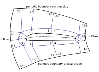
It is chosen to use an O-H grid topology for the rotator section. This can be seen in

figure

2.5 , where the grid around the turbine is an O-grid and the grid around the O-grid

is a H-grid topology. The topology will be extruded in the hub to shroud direction to

form a 3-D grid. The blocks depicted here will be divided into smaller volumes, which

(12)

Chapter 2. Background on meshes

6 Computational Domain

Hub

Shroud

pressure side

suction side

r

z

[image:12.596.93.464.124.300.2]

Rotational axis

Figure 2.4:

Sketch of the computational domain

1

2 3 4

5

6

7

8

9

10

11

12

13

14

15

16

17

18

19

20

21

22

23

24 in

ﬂ

ow

out

ﬂ

ow

periodic boundary pressure side

periodic boundary suction side

[image:12.596.93.472.404.680.2]

(13)

Chapter 3

Mesh generation

3.1 Introduction

During the internship a python script was written that, in cooparation with the Eilmer3

code, creates a structured mesh from a given input. In this chapter this process is

explained step by step, where a more detailed explanation of the code is given in the

appendix

A

.

The overall process is as follows. At first the input will be used to create the surfaces

of the rotor. From that the computational domain is created. Then the computational

domain is subdevided into a structure similar to the one seen in figure

2.5 .

3.2 Input

The input consists of points along the curves describing the pressure and suction side as

well as the camber line of the blade. There are several of these curves at different hub to

shroud locations. These points are made into curves with the Eilmer3 spline function,

which results for example in figure

3.1 for the camberlines of the blade.

(14)

[image:14.596.86.475.86.384.2]

Chapter 3. Mesh generation

8 Figure 3.1:

Camberline curves created from the input

3.3 Loft

From the curves given in the input a surface has to be created. This is done through

lofting and while quite a few options are available to create surfaces with Eilmer3 this

is not one of them. The following process describes how lofting was implemented.

Any continuous surface can be described with two coordinates, as can be seen in figure

3.2 . The surface has an arbitrary distribution of points in the 3D space.

Define

i

and

j

as 0 at the beginning corner and 1 at their respective ends. Now a function

f

(

i, j

) with 0

≥

i

≥

1 and 0

≥

j

≥

1 can describe the surface completely. This is applied

to create a surface from the input curves.

In this case

i

= 0 is the inflow location,

i

= 1 is the outflow location,

j

= 0 is the hub

location and

j

= 1 is the shroud location. Several curves in

i

direction are given in the

input at different

j

positions. To obtain the coordinates of the surface for an arbitrary

combination of

i

and

j

the following is done. Evaluate all input curves at location

i

arbitrary

this will result in one point per input curve. A new curve in the

j

direction is

then created using all these points. Evaluating this curve at its

j

arbitrary

location gives

the coordinates of the surface that one was looking for. The process above can be done

for any combination of

i

and

j

and therefore describes the complete surface.

(15)

Chapter 3. Mesh generation

9

[image:15.596.126.505.84.323.2]

j

i

Figure 3.2:

Sketch of a surface to explain lofting

3.4 Computational Domain

To create a hexahedral volume in the given environment it is sufficient to define all its

six faces. This works in a similar way as described for the surface in the previous section,

where a third computational dimension is added. The structure of these volume blocks

is explained further in appendix

A

section

A.3 .

The whole computational domain is build up out of several blocks as seen in the topology

sketch, figure

2.5 . In the script the whole computational domain is created first by

separately creating six volumes, as seen in figure

3.2 . Their surfaces are then later used

when blocks are created.

The division into volumes is sketched in figure

3.3 where this sketch has to be extruded

in the hub to shroud direction to obtain volumes. It has to be mentioned that the

clearance, the space between rotor and shroud is not yet taken into consideration in this

code.

The surfaces of the volumes are of main interest here, especially the periodic boundaries.

• The hub and shroud surfaces follow from the geometry and can be implemented

straight forward.

• The inflow surface is chosen to be part of a cylinder shell and the outflow surface

is part of a disk.

(16)

Chapter 3. Mesh generation

10

• The periodic boundaries are more complex and are explained below

The periodic boundaries cannot simply be surfaces with a constant azimuthal

coordi-nate. That is because of the curvature of the blades, especially in the outflow section,

which can be seen for example in figure

3.4 . This curvature in combination with an

option to use a large number of blades require a different kind of boundary.

The periodic boundaries consist of three parts, the inflow part belonging to volumes V5

and V6, the rotator part belonging to volume V1 and V4 and the outflow part

belong-ing to V2 and V3. The inflow part flat surfaces with constant azimuthal position. The

rotator part is a lofted surface created from rotated camberline curves. The outflow

part of the periodic boundary is then created in a way that it smoothly connects to the

camberline surface of V1 and V4. This is done by matching the slope

_∂z

∂θ

of both surfaces

at their connection.

With all surfaces the computational domain is defined as seen in figure

3.5 and the

cre-ation of the grid can begin.

in

ﬂ

ow

out

ﬂ

ow

periodic boundary pressure side

periodic boundary suction side

V1

V2

V3

V4

V5

V6

azimuthal direction

[image:16.596.93.470.370.603.2]

θ

(17)

[image:17.596.129.503.100.238.2]

Chapter 3. Mesh generation

11 Figure 3.4:

Photo of a rotator section of a radial inflow turbine

Blade

in

ﬂ

ow direction

out

ﬂ

ow direction

[image:17.596.128.503.313.710.2]

(18)

Chapter 3. Mesh generation

12

3.5 Creation of the Topology

A sketch of the topology is given in figure

2.5 . One has to keep in mind, that this is

sketch of a cut through the volume at a hub to shroud location. Therefore the surface is

not just 2D as displayed here, it actually follows the hub, inflow and outflow geometry.

Thus the following operations seem straight forward but are complicated by the fact

that they have to be done in the respective working surface.

The remaining lines (surfaces when extruded) that still need to be created are displayed

blue in figure

2.5 . First an O-grid line is created which has a constant distance to the

blade. Then nodes are distributed over the inflow and outflow lines, over the periodic

boundaries and over the O-grid line. These are then connected. This is done in a way

that can easily be adapted, so that the number of blocks can be increased and their

node position can be changed, see appendix

A

section

A.5.1 .

The resulting distribution in 3D can be seen in figure

3.6 .

Blade

[image:18.596.109.435.333.704.2]

in

ﬂ

ow direction

out

ﬂ

ow direction

(19)

Chapter 4

Summary

A script has been created to automatically create an OH-grid type structured mesh

around blades of the rotor of an radial inflow turbine.

A way to loft a surface from a given set of curves has been found, which can easily be

implemented into the Eilmer3 code and can be used for for many different applications.

The challenging geometry has been devided into an OH-grid type structure, where blocks

are created automatically and the number of blocks and their location can be adjusted

by changing very few input parameters.

The distribution of the cells along the boundaries still has to be adjusted to capture

the boundary layer for example. Currently the cells are evenly divided along the block

boundaries. Once this is achieved an automated process can be run to solve CFD

cal-culations on this grid.

Another feature that might need to be added to the script is the ability to model the

clearance in between blade and shroud.

Functions used in the code can be reused to create scripts for automatic mesh generation

stators or other geometries.

(20)

(21)

Appendix A

Code explanations

In this appendix the script is explained in more detail. This includes an explanation of

how to work with the script and which lines are responsible for what operation. Overall

the script is run with the data preparation tool of Eilmer3. Command:

$

e

3 prep.py

− −

job

=

jobname

The input that is required consists of “.obj” files containing curves on the pressure side,

suction side and the camberline of the blade. These files need to be ordered in hub to

shroud direction and they should start at the leading edge and end at the trailing edge.

Next to the curves given in the input also the number of blades has to be defined, as

well as the inflow and outflow length. This will determine the size of the computational

domain.

In general only the file location and number of blade has to be given and the rest is done

automatically. For further fine-tuning see the different sections in this appendix.

During the code creation the pressure and suction side did not start at the leading and

trailing edge therefore only the camberlines were used. Once this is implemented certain

curves in this code have to be changed, most importantly Volume lines (line 158,337),

and lines 880 - 882,1101 have match the correct geometries.

A.1 Input interpreter

The location of the input curves is determined in code lines 20 to 34. These have to be

changed to be able to run the script. The “loader” function and the “input interpreter”

function are used together to create splines from the input.

They make use of the structure of the “.obj” file to extract data points. A spline using

the Eilmer3 spline function is then created through every point per curve.

(22)

Appendix A.

Code explanations

16

A.2 Loft

The idea behind lofting is explained is section

3.3 . This procedure can be implemented

into the current Eilmer3 environment using only 20 lines of code, see the “Loft” function

in the python script, which is the input to the already existing “PyFunctionSurface” in

Eilmer3 to create a lofted surface.

It evaluates all input curves at the desired

i

location and creates a spline through all

these points. This spline will then be evaluated at the desired

j

location and thus the

Cartesian coordinates for any combination of

i

and

j

can be obtained.

However, this function assumes that the curves are given in the same

i

direction and

that they follow a strict order in the

j

direction otherwise the resulting surface does

not make sense. Furthermore in case of the radial inflow turbine the coordinates are

assumed to be such, that the center axis is in the z direction and goes through the origin

of a Cartesian coordinate system.

A.3 Computational domain

The arrangement of volumes is shown in figure

3.3 . In Eilmer3 the volumes are arranged

as displayed in

A.1 . The code is generated in a way, that the top face corresponds with

the shroud, the bottom face corresponds with the hub, the west surface belongs to the

inflow direction and the east surface belongs to the outflow direction.

[image:22.596.88.467.492.698.2]

The volumes are created in the code in lines 155 to 645.

(23)

Appendix A.

Code explanations

17

A.4 Automated block creation

A more detailed sketch of the topology is given in figure

A.2 . It contains the

nomencla-ture used in the code. The following parts will explain how the remaining surfaces are

created.

1 ₂

_{3 4}

5

6

7

8

9

10

11

12

13

14

15

16

17

18

19

20

21

22

23

24 in

ﬂ

ow

H-blocks

out

H-blocks

ﬂ

ow

suction side H-blocks

O-grid line

pressure side H-blocks

in

ﬂ

ow

corner blocks

in

ﬂ

ow

[image:23.596.127.509.177.364.2]

corner blocks

Figure A.2:

Sketch of the structure of the computational domain

A.4.1 O-grid surface

The part of the code that is responsible for creating the O-grid surfaces is given in lines

655 to 888.

The O-grid line is created in the following way:

At 120 locations along the input curve points are created at a fixed distance to the blade

(adjustable through

number of points for ogl

and

distance ogl blade

). It is made

sure that these points lie on the working surface.

Through these points a curve is created to obtain a O-grid line. Then all the O-grid

lines are lofted to create an O-grid surface.

A.4.2 Connection between nodes

The function

simple connector

(lines 911 to 1096) creates a curve connecting two

nodes. This curve is part of the working surface. The connecting surface is then

cre-ated using its four surrounding paths (two times path on surface and two times simple

(24)

Appendix A.

Code explanations

18

A.4.3 Automated block creation functions

With the O-grid surface defined and the ability to connect nodes, automated functions

are written to automatically create blocks (lines 1130 to 1945). Here a distinction is made

between inflow H-blocks (

create In Block

), periodic side H-blocks (

create H Block

),

outflow H-blocks (

create Out Block

), O-grid blocks (

create O Block

) and corner blocks,

see sketch

A.2 .

A.5 Grid creation

Using all the functions described above the complete grid can be created starting with the

pressure side of the computational domain (lines 2092 to 2303). First the inflow H-blocks

are created, followed by the inflow corner block then the periodic H-blocks, afterwards

the outflow corner block is created and then the outflow H-blocks are created. Finally

the blocks in the O-grid section are created. This process is repeated for the suction

side.

The number of blocks created depends on the number of nodes defined along each

curve. Thus changing the location and number of the nodes defines the topology of the

computational domain. A preliminary selection of node locations has been done for the

given geometry and is given in the next section. However, the location and number of

nodes might have to be changed for different geometries.

A final adjustment that has to be made by the user is to activate the block creation parts

in the code that are currently commented and include cluster functions to distribute the

nodes along each block.

A.5.1 Node location

Node locations are chosen along the periodic boundaries, the blade, the O-grid surface,

the inflow surface and the outflow surface. Here 0 stands for the beginning of the surface

and 1 for its end. The directions are shown in figure

A.2 .

The following node locations were chosen to produce figure

3.6 they can be found in

the code at lines 1962 to 2074. A note of caution: When the number of inlet or outlet

H-blocks is changed the corresponding node on the O-grid line has to be changed, see

lines 2071 to 2074.

1 N o d e s o n B l a d e p r e s s u r e = [ 0 , 0 . 0 3 , 0 . 1 , 0 . 2 , 0 . 3 , 0 . 4 , 0 . 5 , 0 . 6 , 0 . 6 5 , 0 . 7 , 0 . 8 5 , 0 . 9 , 0 . 9 8 , 1 ] 2 N o d e s o n B l a d e s u c t i o n = [ 0 , 0 . 0 3 , 0 . 1 , 0 . 2 , 0 . 3 , 0 . 4 , 0 . 5 , 0 . 6 , 0 . 6 5 , 0 . 7 5 , 0 . 8 5 , 0 . 8 8 , 0 . 9 8 , 1 ] 3 N o d e s o n o g r i d l i n e p r e s s u r e = [ 0 , 0 . 0 3 , 0 . 1 , 0 . 2 , 0 . 3 , 0 . 4 , 0 . 5 , 0 . 6 , 0 . 6 5 , 0 . 7 , 0 . 8 5 , 0 . 9 , 0 . 9 8 , 1 ] 4 N o d e s o n o g r i d l i n e s u c t i o n = [ 0 , 0 . 0 3 , 0 . 1 , 0 . 2 , 0 . 3 , 0 . 4 , 0 . 5 , 0 . 6 , 0 . 6 5 , 0 . 7 , 0 . 8 2 , 0 . 9 , 0 . 9 6 , 1 ] 5 N o d e s o n i n l e t p r e s s u r e = [ 0 . 9 , 1 ]

(25)

Appendix A.

Code explanations

19

7 N o d e s o n p e r i o d i c p r e s s u r e = [ 0 . 1 5 , 0 . 2 8 , 0 . 3 6 , 0 . 4 , 0 . 4 4 , 0 . 4 7 5 , 0 . 5 , 0 . 5 5 , 0 . 5 7 , 0 . 6 0 , 0 . 6 2 , 0 . 6 5 ] 8 N o d e s o n p e r i o d i c s u c t i o n = [ 0 . 1 5 , 0 . 2 8 , 0 . 3 6 , 0 . 4 , 0 . 4 4 , 0 . 4 7 5 , 0 . 5 , 0 . 5 5 , 0 . 6 0 , 0 . 6 2 , 0 . 7 , 0 . 9 ] 9 N o d e s o n o u t l e t p r e s s u r e = [ 0 . 9 , 1 ]

10 N o d e s o n o u t l e t s u c t i o n = [ 0 . 0 , 0 . 4 ]

A.6 Visualisation

During the creation of the script intermediate results had to be visualized. This is done

both to check for failures in the code and to determine the location of certain blocks.

The preferred way to do this is with the Blender [

5 ] software. First the mesh

genera-tion script is used to create text files containing coordinates of points along curves that

should be displayed. These text files should have the following structure:

1 x1 y1 z 1 2 x2 y2 z 2 3 . . .

In the code this is generally done by appending curve elements to the list of A. At the

end of the code all curves contained in that list are written to separate text files.

Then Blender can be started in scripting mode. Use the script below where the file

location and number of curves of to be changed. Run the script and it will load and

display the desired curves.

1 ## Run t h i s s c r i p t i n b l e n d e r and i t w i l l c r e a t e and d i s p l a y c u r v e s

2 ## t h a t come f r o m i n p u t f i l e s c o n t a i n o n l y x , y and z c o o r d i n a t e s o f p o i n t s ( o n e p o i n t p e r l i n e ) .

3 ## J u s t c h a n g e t h e f i l e l o c a t i o n and number o f c u r v e s and p r e s s r u n . Then t h e c u r v e s w i l l be d i s p l a y e d .

4

5 i m p o r t bpy

6 f r o m m a t h u t i l s i m p o r t V e c t o r 7

8 w= 1 # w e i g h t j u s t l e a v e t h i s a s 1

9 n u m b e r o f c u r v e s = 10 # g i v e s t h e number o f c u r v e s t h a t a r e l o a d e d i n t o b l e n d e r

10

11 f o r n i n r a n g e ( 0 ,n u m b e r o f c u r v e s) : 12 c L i s t = None

13 c L i s t = [ ] 14

15 f o r l i n e i n open(” / f i l e l o c a t i o n / f i l e %d . t x t ”%n, ” r ”) : ## c h a n g e t h i s t o t h e p r o p e r f i l e l o c a t i o n

16 v a l s = l i n e.s p l i t( ) 17 x = f l o a t(v a l s[ 0 ] ) 18 y = f l o a t(v a l s[ 1 ] ) 19 z = f l o a t(v a l s[ 2 ] )

20 c L i s t.append(V e c t o r( (x,y,z) ) ) 21

22

23 c u r v e d a t a = bpy.d a t a.c u r v e s.new(name=’ Curve ’, t y p e=’CURVE ’) 24 c u r v e d a t a.d i m e n s i o n s = ’ 3D ’

25

26 o b j e c t d a t a = bpy.d a t a.o b j e c t s.new(” ObjCurve ”, c u r v e d a t a) 27 o b j e c t d a t a.l o c a t i o n = ( 0 , 0 , 0 ) #o b j e c t o r i g i n

28 bpy.c o n t e x t.s c e n e.o b j e c t s.l i n k(o b j e c t d a t a) 29

(26)

Appendix A.

Code explanations

20

32 f o r num i n r a n g e(l e n(c L i s t) ) : 33 x, y, z = c L i s t[num]

(27)

Appendix B

Mesh generation code

The whole code to generate the mesh

1 j o b t i t l e = ” C r e a t i n g t h e mesh . . . ” 2 p r i n t j o b t i t l e

3

4 # A c c e p t d e f a u l t s f o r a i r g i v i n g R= 2 8 7 . 1 , gamma=1.4

5 s e l e c t g a s m o d e l(model=’ i d e a l g a s ’, s p e c i e s=[’ a i r ’] ) 6

7 i n i t i a l C o n d = F l o w C o n d i t i o n(p= 1 0 0 0 . 0 , u= 0 . 0 , T= 3 0 0 . 0 ) 8 M i n f = 4 . 0

9 u i n f = M i n f ∗ i n i t i a l C o n d.f l o w.g a s.a

10 i n f l o w C o n d = F l o w C o n d i t i o n(p= 5 0 . 0e3, u=u i n f , T= 3 0 0 . 0 ) 11

12

13 #################### i n p u t n e e d e d f o r g e o m e t r y

14

15 n u m b e r o f b l a d e s = 12 #f o r now 3 b l a d e s n o t w o r k i n g d o n t know why : / e v e r y t h i n g e l s e i s

16 c l e a r a n c e = 0 . 0 2 #n o t i m p l e m e n t e d y e t

17 i n f l o w s p a c e = 0 . 0 5 #t h i s f a c t o r t i m e s t h e c a m b e r l i n e l e n g t h g i v e s t h e i n f l o w l e n g t h

18 o u t f l o w s p a c e = 0 . 0 5 19

20 f i l e c a m b e r h u b = ” / f i l e l o c a t i o n / o b j 3 D h u b . o b j ”

21 f i l e c a m b e r h u b t o s h r o u d = ” / f i l e l o c a t i o n / o b j 3 D h u b S h r o u d I n t e r m e d i a t e L i n e%d . o b j ” 22 n u m b e r o f i n t e r m e d i a t e c a m b e r f i l e s = 20

23 f i l e c a m b e r s h r o u d = ” / f i l e l o c a t i o n / o b j 3 D s h r o u d . o b j ” 24

25

26 f i l e p r e s s u r e s i d e h u b = ” / f i l e l o c a t i o n / o b j 3 D h u b s i d e 2 . o b j ”

27 f i l e p r e s s u r e s i d e h u b t o s h r o u d = ” / f i l e l o c a t i o n / o b j 3 D h u b S h r o u d I n t e r m e d i a t e s p r e s s u r e S i d e% d . o b j ”

28 n u m b e r o f i n t e r m e d i a t e p r e s s u r e f i l e s = 20

29 f i l e p r e s s u r e s i d e s h r o u d = ” / f i l e l o c a t i o n / o b j 3 D s h r o u d s i d e 2 . o b j ” 30

31 f i l e s u c t i o n s i d e h u b = ” / f i l e l o c a t i o n / o b j 3 D h u b s i d e 1 . o b j ”

32 f i l e s u c t i o n s i d e h u b t o s h r o u d = ” / f i l e l o c a t i o n / o b j 3 D h u b S h r o u d I n t e r m e d i a t e s s u c t i o n S i d e%d . o b j ”

33 n u m b e r o f i n t e r m e d i a t e s u c t i o n f i l e s = 20

34 f i l e s u c t i o n s i d e s h r o u d = ” / f i l e l o c a t i o n / o b j 3 D s h r o u d s i d e 1 . o b j ” 35

36 ###################################### F i l e l o a d e r

37 d e f l o a d e r(f i l e n a m e,n u m b e r o f f i l e s) : ### l o a d . o b j f i l e s t h a t a r e o r d e r e d by numbers e . g . f i l e n a m e 1 f i l e n a m e 2 . . . f o r number o f f i l e s = 0 i t j u s t l o a d s t h e f i l e f i l e n a m e

38 v e r t s= [ ] ### i n p u t e x a m p l e : f i l e n a m e = ” o b j 3 D h u b S h r o u d I n t e r m e d i a t e L i n e%d . o b j ”

39 i f n u m b e r o f f i l e s == 0 :

40 f o r l i n e i n open(f i l e n a m e, ” r ”) : 41 v a l s = l i n e.s p l i t( )

42 i f v a l s[ 0 ] == ” v ”:

43 v= map(f l o a t, v a l s[ 1 : 4 ] )

(28)

Appendix A.

Code explanations

22

44 v e r t s.append(v) 45 e l s e:

46 f o r l i n e i n open(f i l e n a m e %n u m b e r o f f i l e s, ” r ”) : 47 v a l s = l i n e.s p l i t( )

48 i f v a l s[ 0 ] == ” v ”:

49 v = map(f l o a t, v a l s[ 1 : 4 ] ) 50 v e r t s.append(v)

51

52 r e t u r n v e r t s 53

54 #################################### C r e a t e i n p u t c u r v e s f r o m g i v e n f i l e s i n t h e o r d e r : Hub , hub t o s h r o u d i n t e r m e d i a t e s , Shroud . A l l a r e l o c a t e d i n i n p u t c u r v e s

55 #################################### The c u r v e s t a r t s a t t h e i n f l o w b l a d e , e n d s a t o u t f l o w o f b l a d e

56 d e f i n p u t i n t e r p r e t e r(h u b l o c a t i o n,h u b t o s h r o u d l o c a t i o n,s h r o u d l o c a t i o n, n u m b e r o f i n b e t w e e n f i l e s) :

57 i n p u t c u r v e s= [ ] 58 dummy= [ ] 59

60 l i n e c o o r d s = l o a d e r(h u b l o c a t i o n, 0 ) ### l o a d a l l t h e p o i n t s f r o m o n e f i l e , t h e n c r e a t e a s p l i n e t h r o u g h i t

61 f o r i i n r a n g e( 0 ,l e n(l i n e c o o r d s) ) :

62 dummy.append(V e c t o r(l i n e c o o r d s[i] [ 0 ] ,l i n e c o o r d s[i] [ 1 ] ,l i n e c o o r d s[i] [ 2 ] ) ) 63 i n p u t c u r v e s.append(S p l i n e(dummy) )

64 65

66 f o r n i n r a n g e( 1 ,n u m b e r o f i n b e t w e e n f i l e s+1) : 67 Q=None

68 Q= [ ]

69 l i n e c o o r d s=l o a d e r(h u b t o s h r o u d l o c a t i o n,n) 70 f o r i i n r a n g e( 0 ,l e n(l i n e c o o r d s) ) :

71 Q.append(V e c t o r(l i n e c o o r d s[i] [ 0 ] ,l i n e c o o r d s[i] [ 1 ] ,l i n e c o o r d s[i] [ 2 ] ) ) 72 i n p u t c u r v e s.append(S p l i n e(Q) )

73

74 dummy=None 75 dummy= [ ]

76 l i n e c o o r d s = l o a d e r(s h r o u d l o c a t i o n, 0 ) 77 f o r i i n r a n g e( 0 ,l e n(l i n e c o o r d s) ) :

78 dummy.append(V e c t o r(l i n e c o o r d s[i] [ 0 ] ,l i n e c o o r d s[i] [ 1 ] ,l i n e c o o r d s[i] [ 2 ] ) ) 79 i n p u t c u r v e s.append(S p l i n e(dummy) )

80

81 r e t u r n i n p u t c u r v e s 82

83

84 ################################### D e f i n e L o f t s u r f a c e . . . r = 0 i n f l o w r = 1 o u t f l o w , s = 0 hub s = 1 s h r o u d

85 ################################### P y S u r f a c e o n l y a l l o w s 2 i n p u t s . . t h e r e f o r e make s u r e you c a l l i n p u t c u r v e s = i n p u t i n t e r p r e t e r ( hub , h t s , s h r o u d , NoF ) f i r s t !

86 ################################### e x a m p l e : i n p u t c u r v e s = i n p u t i n t e r p r e t e r ( f i l e c a m b e r h u b , f i l e c a m b e r h u b t o s h r o u d , f i l e c a m b e r s h r o u d ,

n u m b e r o f i n t e r m e d i a t e c a m b e r f i l e s )

87 ################################### d e s i r e d l o f t e d s u r f a c e = P y F u n c t i o n S u r f a c e ( L o f t U s e r D e f i n e d )

88 ################# Volume 1

89

90 i n p u t c u r v e s = i n p u t i n t e r p r e t e r(f i l e c a m b e r h u b,f i l e c a m b e r h u b t o s h r o u d,f i l e c a m b e r s h r o u d, n u m b e r o f i n t e r m e d i a t e c a m b e r f i l e s)

91

92 d e f L o f t(i n p u t c u r v e s) : 93 i n p u t c u r v e s s s = [ ]

94 f o r i i n r a n g e ( 0 ,l e n(i n p u t c u r v e s) ) :

95 i n p u t c u r v e s s s.append(i n p u t c u r v e s[i] .c l o n e( ) ) 96 d e f L o f t U s e r D e f i n e d(r,s) :

97

98 Q=None 99 Q= [ ] 100

101 r C u r v e s=i n p u t c u r v e s s s 102

103 f o r n i n r a n g e( 0 ,l e n(r C u r v e s) ) : 104 Q.append(r C u r v e s[n] .e v a l(r) ) 105

(29)

Appendix A.

Code explanations

23

109 r e t u r n (C o o r d s.x,C o o r d s.y,C o o r d s.z) 110 r e t u r n L o f t U s e r D e f i n e d

111 112

113 ################################### r o t a t e t h e l o f t e d s u r f a c e c o u n t e r c l o c k w i s e a r o u n d z BE CAREFULL ABOUT i n p u t c u r v e s ! !

114

115 d e f L o f t R o t a t o r(i n p u t c u r v e s) : 116 i n p u t c u r v e s s s = [ ]

120

121 Q=None 122 Q= [ ] 123

129 s C u r v e=S p l i n e(Q) 130 C o o r d s = s C u r v e.e v a l(s) 131

132 r e t u r n (C o o r d s.x,C o o r d s.y,C o o r d s.z) 133

134 d e f L o f t R o t a t e(r,s) :

135 f r o m math i m p o r t c o s, s i n, p i 136

137 t h e t a = 2 ∗ p i / n u m b e r o f b l a d e s ∗1 / 2 #o n l y r o t a t e h a l f t h e a n g l e b u t i n b o t h d i r e c t i o n s o f c o u r s e . . . . =.=

138 c c = c o s (t h e t a) 139 s s = s i n (t h e t a) 140

141 C o o r d s = L o f t U s e r D e f i n e d(r,s) 142 x = C o o r d s[ 0 ]

143 y = C o o r d s[ 1 ] 144 z = C o o r d s[ 2 ] 145 x r = x∗c c−y∗s s 146 y r=x∗s s+y∗c c 147

148 r e t u r n (x r,y r,z) 149

150 r e t u r n L o f t R o t a t e 151

152

153 ###################################

154 ################################### F i r s t Volume a c c o r d i n g t o my d e f i n i t i o n o f t o p b o t e t c .

155 p r i n t(” Volume1###############################”) 156

157 #n o r t h = P y F u n c t i o n S u r f a c e ( L o f t U s e r D e f i n e d )

158 n o r t h = P y F u n c t i o n S u r f a c e(L o f t(i n p u t c u r v e s) ) 159 #s o u t h = P y F u n c t i o n S u r f a c e ( L o f t R o t a t e )

160 s o u t h = P y F u n c t i o n S u r f a c e(L o f t R o t a t o r(i n p u t c u r v e s) ) 161

162 p2 = n o r t h.e v a l( 1 . 0 , 0 . 0 ) 163 p3 = n o r t h.e v a l( 0 . 0 , 0 . 0 ) 164 p6 = n o r t h.e v a l( 1 . 0 , 1 . 0 ) 165 p7 = n o r t h.e v a l( 0 . 0 , 1 . 0 ) 166

167 p0 = s o u t h.e v a l( 0 . 0 , 0 . 0 ) 168 p1 = s o u t h.e v a l( 1 . 0 , 0 . 0 ) 169 p4 = s o u t h.e v a l( 0 . 0 , 1 . 0 ) 170 p5 = s o u t h.e v a l( 1 . 0 , 1 . 0 ) 171

172 # p r i n t ” p0 =” , p0 , ” p1 =” , p1

173 174 175

176 p r i n t(” t o p ”)

177 c 5 6 = Arc(p5, p6,V e c t o r( 0 , 0 ,p5.z) ) 178 c 4 7 = Arc(p4, p7,V e c t o r( 0 , 0 ,p4.z) )

(30)

Appendix A.

Code explanations

24

182 183

184 p r i n t(” b o t t o m ”)

185 c 0 3 = Arc(p0, p3,V e c t o r( 0 , 0 ,p0.z) ) 186 c 1 2 = Arc(p1, p2,V e c t o r( 0 , 0 ,p1.z) )

187 c 0 1 = P a t h O n S u r f a c e(s o u t h, L i n e a r F u n c t i o n( 1 . 0 , 0 . 0 ) , L i n e a r F u n c t i o n( 0 . 0 , 0 . 0 ) ) 188 c 3 2 = P a t h O n S u r f a c e(n o r t h, L i n e a r F u n c t i o n( 1 . 0 , 0 . 0 ) , L i n e a r F u n c t i o n( 0 . 0 , 0 . 0 ) ) 189 bottom = CoonsPatch(c01, c32, c03, c12, ” bottom ”)

190 191

192 p r i n t(” w e s t ”)

193 c 3 7 = P a t h O n S u r f a c e(n o r t h, L i n e a r F u n c t i o n( 0 . 0 , 0 . 0 ) , L i n e a r F u n c t i o n( 1 . 0 , 0 . 0 ) ) 194 c 0 4 = P a t h O n S u r f a c e(s o u t h, L i n e a r F u n c t i o n( 0 . 0 , 0 . 0 ) , L i n e a r F u n c t i o n( 1 . 0 , 0 . 0 ) ) 195 w e s t = CoonsPatch(c03, c47, c04, c37,” w e s t ”)

196 197

198 p r i n t(” e a s t ”)

199 c 2 6 = P a t h O n S u r f a c e(n o r t h, L i n e a r F u n c t i o n( 0 . 0 , 1 . 0 ) , L i n e a r F u n c t i o n( 1 . 0 , 0 . 0 ) ) 200 c 1 5 = P a t h O n S u r f a c e(s o u t h, L i n e a r F u n c t i o n( 0 . 0 , 1 . 0 ) , L i n e a r F u n c t i o n( 1 . 0 , 0 . 0 ) ) 201 e a s t = CoonsPatch(c12, c56, c15, c26,” e a s t ”)

202 203

204 pvolume = P a r a m e t r i c V o l u m e(n o r t h, e a s t, s o u t h, w e s t, top, bottom, ” P r e s s u r e s i d e v o l u m e ”) 205

206

207 #b l k 1 = Block3D ( l a b e l =” f i r s t−b l o c k ” , n n i =20 , n n j =20 , nnk =20 ,

208 # p a r a m e t r i c v o l u m e=pvolume ,

209 # f i l l c o n d i t i o n =i n i t i a l C o n d )

210 #b l k 1 . s e t B C ( ”WEST” , ” SUP IN ” , i n f l o w c o n d i t i o n=i n f l o w C o n d )

211 #b l k 1 . s e t B C ( ”SOUTH” , ”SUP OUT” )

212 #b l k 1 . s e t B C ( ”TOP” , ”SUP OUT” )

213 #b l k 1 . s e t B C ( ”BOTTOM” , ”SUP OUT” )

214 215

216 ################################### Volume number 6 a c c o r d i n g t o my i n t e r m e d i a t e n o m e n c l a t u r e , i n l f o w p r e s s u r e b l o c k

217 ################################### E x t r u d e f o r i n f l o w INPUT CURVES ! ! ! ! WARNING 2 s o l u t i o n s f o r x and y c a u s e o f s q r t . . . : /

218 p r i n t(” Volume6################################”) 219

220 d e f e x t r u d e(p o i n t,e x t r u d e l e n g t h) : 221 f r o m math i m p o r t s q r t

222

223 x = p o i n t.x 224 y = p o i n t.y 225 z = p o i n t.z 226

227 r 2 = s q r t(x∗∗2+y∗ ∗2 )+e x t r u d e l e n g t h 228 a = x / y

229

230 y = s q r t(r 2∗∗2/(1+a∗ ∗2 ) ) 231 x = y∗a

232

233 r e t u r n V e c t o r(x,y,z) 234

235 v6p2 = p3

236 v6p3 = e x t r u d e(p3,i n f l o w s p a c e∗i n p u t c u r v e s[ 0 ] .l e n g t h( ) ) 237 v6p6 = p7

238 v6p7 = V e c t o r(v6p3.x,v6p3.y,v6p6.z) 239

240 v6p0 = e x t r u d e(p0,i n f l o w s p a c e∗i n p u t c u r v e s[ 0 ] .l e n g t h( ) ) 241 v6p1 = p0

242 v6p5 = p4

243 v6p4 = V e c t o r(v6p0.x,v6p0.y,v6p5.z) 244

245 #p r i n t ” v6p4 =” , v6p4 , ” v6p5 =” , v6p5 , ” v6p6 =” , v6p6 , ” v6p7 =” , v6p7

246 #p r i n t ” v6p0 =” , v6p0 , ” v6p1 =” , v6p1 , ” v6p2 =” , v6p2 , ” v6p3 =” , v6p3

247 248

249 p r i n t(” v 6 t o p ”)

250 v 6 c 5 6 = c 4 7

251 v 6 c 4 5 = L i n e(v6p4,v6p5) 252 v 6 c 7 6 = L i n e(v6p7,v6p6)

253 v 6 c 4 7 = Arc(v6p4,v6p7,V e c t o r( 0 , 0 ,v6p4.z) )

(31)

Appendix A.

Code explanations

25

255 #

256 257

258 p r i n t(” v 6 b o t t o m ”) 259 v 6 c 0 3 = Arc(v6p0, v6p3,V e c t o r( 0 , 0 ,v6p0.z) )

260 v 6 c 1 2 = c 0 3

263 v6bottom = CoonsPatch(v 6 c 0 1, v 6 c 3 2, v 6 c 0 3, v 6 c 1 2, ” v6bottom ”) 264 #

265 #

266 p r i n t(” v 6 w e s t ”)

269 v 6 w e s t = CoonsPatch(v 6 c 0 3, v 6 c 4 7, v 6 c 0 4, v 6 c 3 7,” v 6 w e s t ”) 270 #

271 #

272 p r i n t(” v 6 e a s t ”)

273 v 6 c 2 6 = c 3 7 274 v 6 c 1 5 = c 0 4

275 #v 6 e a s t = CoonsPatch ( v 6 c 1 2 , v 6 c 5 6 , v 6 c 1 5 , v 6 c 2 6 , ” v 6 e a s t ” )

276 v 6 e a s t = w e s t 277

278 p r i n t(” v 6 n o r t h ”)

279 v 6 n o r t h = CoonsPatch(v 6 c 3 2, v 6 c 7 6, v 6 c 3 7, v 6 c 2 6, ” v 6 n o r t h ”) 280

281 p r i n t(” v 6 s o u t h ”)

282 v 6 s o u t h = CoonsPatch(v 6 c 0 1, v 6 c 4 5, v 6 c 0 4, v 6 c 1 5, ” v 6 s o u t h ”) 283

284 285 286

287 v6pvolume = P a r a m e t r i c V o l u m e(v 6 n o r t h, v 6 e a s t, v 6 s o u t h, v 6 w e s t, v 6 t o p, v6bottom, ” I n f l o w P r e s s u r e s i d e b l o c k ”)

288

289 #b l k 6 = Block3D ( l a b e l =” b l o c k 6 ” , n n i =20 , n n j =20 , nnk =20 ,

290 # p a r a m e t r i c v o l u m e=v6pvolume ,

292 293

294 ################################### B l o c k number 4 a c c o r d i n g t o my i n t e r m e d i a t e n o m e n c l a t u r e , s u c t i o n s i d e b l o c k

295 ################################### INPUT CURVES ! ! ! !

296 p r i n t(” Volume4################################”)

298

299 d e f L o f t R o t a t o r C l o c k w i s e(i n p u t c u r v e s) : 300 i n p u t c u r v e s s s = [ ]

304

305 Q=None 306 Q= [ ] 307

313 s C u r v e=S p l i n e(Q) 314 C o o r d s = s C u r v e.e v a l(s) 315

316 r e t u r n (C o o r d s.x,C o o r d s.y,C o o r d s.z) 317

318 d e f L o f t R o t a t e C l o c k w i s e(r,s) : 319 f r o m math i m p o r t c o s, s i n, p i 320

321 t h e t a = −2 ∗ p i / n u m b e r o f b l a d e s ∗1 / 2 322 c c = c o s (t h e t a)

323 s s = s i n (t h e t a) 324

(32)

Appendix A.

Code explanations

26

327 y = C o o r d s[ 1 ] 328 z = C o o r d s[ 2 ] 329 x r = x∗c c−y∗s s 330 y r=x∗s s+y∗c c 331

332 r e t u r n (x r,y r,z) 333

334 r e t u r n L o f t R o t a t e C l o c k w i s e 335

336 v 4 n o r t h = P y F u n c t i o n S u r f a c e(L o f t R o t a t o r C l o c k w i s e(i n p u t c u r v e s) ) 337 v 4 s o u t h = P y F u n c t i o n S u r f a c e(L o f t(i n p u t c u r v e s) )

338

339 #v 4 n o r t h = P y F u n c t i o n S u r f a c e ( L o f t R o t a t e C l o c k w i s e )

340 #v 4 s o u t h = P y F u n c t i o n S u r f a c e ( L o f t U s e r D e f i n e d )

341

342 v4p2 = v 4 n o r t h.e v a l( 1 . 0 , 0 . 0 ) 343 v4p3 = v 4 n o r t h.e v a l( 0 . 0 , 0 . 0 ) 344 v4p6 = v 4 n o r t h.e v a l( 1 . 0 , 1 . 0 ) 345 v4p7 = v 4 n o r t h.e v a l( 0 . 0 , 1 . 0 ) 346

347 v4p0 = v 4 s o u t h.e v a l( 0 . 0 , 0 . 0 ) 348 v4p1 = v 4 s o u t h.e v a l( 1 . 0 , 0 . 0 ) 349 v4p4 = v 4 s o u t h.e v a l( 0 . 0 , 1 . 0 ) 350 v4p5 = v 4 s o u t h.e v a l( 1 . 0 , 1 . 0 ) 351

352 # p r i n t ” p0 =” , p0 , ” p1 =” , p1

353 354 355

356 p r i n t(” v 4 t o p ”)

357 v 4 c 5 6 = Arc(v4p5, v4p6,V e c t o r( 0 , 0 ,v4p5.z) ) 358 v 4 c 4 7 = Arc(v4p4, v4p7,V e c t o r( 0 , 0 ,v4p4.z) )

359 v 4 c 7 6 = P a t h O n S u r f a c e(v 4 n o r t h, L i n e a r F u n c t i o n( 1 . 0 , 0 . 0 ) , L i n e a r F u n c t i o n( 0 . 0 , 1 . 0 ) ) 360 v 4 c 4 5 = P a t h O n S u r f a c e(v 4 s o u t h, L i n e a r F u n c t i o n( 1 . 0 , 0 . 0 ) , L i n e a r F u n c t i o n( 0 . 0 , 1 . 0 ) ) 361 v 4 t o p = CoonsPatch(v 4 c 4 5, v 4 c 7 6, v 4 c 4 7, v 4 c 5 6, ” v 4 t o p ”)

362 363

366 v 4 c 1 2 = Arc(v4p1, v4p2,V e c t o r( 0 , 0 ,v4p1.z) )

367 v 4 c 0 1 = P a t h O n S u r f a c e(v 4 s o u t h, L i n e a r F u n c t i o n( 1 . 0 , 0 . 0 ) , L i n e a r F u n c t i o n( 0 . 0 , 0 . 0 ) ) 368 v 4 c 3 2 = P a t h O n S u r f a c e(v 4 n o r t h, L i n e a r F u n c t i o n( 1 . 0 , 0 . 0 ) , L i n e a r F u n c t i o n( 0 . 0 , 0 . 0 ) ) 369 v4bottom = CoonsPatch(v 4 c 0 1, v 4 c 3 2, v 4 c 0 3, v 4 c 1 2, ” v4bottom ”)

370 371

372 p r i n t(” v 4 w e s t ”)

373 v 4 c 3 7 = P a t h O n S u r f a c e(v 4 n o r t h, L i n e a r F u n c t i o n( 0 . 0 , 0 . 0 ) , L i n e a r F u n c t i o n( 1 . 0 , 0 . 0 ) ) 374 v 4 c 0 4 = P a t h O n S u r f a c e(v 4 s o u t h, L i n e a r F u n c t i o n( 0 . 0 , 0 . 0 ) , L i n e a r F u n c t i o n( 1 . 0 , 0 . 0 ) ) 375 v 4 w e s t = CoonsPatch(v 4 c 0 3, v 4 c 4 7, v 4 c 0 4, v 4 c 3 7,” v 4 w e s t ”)

376 377

378 p r i n t(” v 4 e a s t ”)

379 v 4 c 2 6 = P a t h O n S u r f a c e(v 4 n o r t h, L i n e a r F u n c t i o n( 0 . 0 , 1 . 0 ) , L i n e a r F u n c t i o n( 1 . 0 , 0 . 0 ) ) 380 v 4 c 1 5 = P a t h O n S u r f a c e(v 4 s o u t h, L i n e a r F u n c t i o n( 0 . 0 , 1 . 0 ) , L i n e a r F u n c t i o n( 1 . 0 , 0 . 0 ) ) 381 v 4 e a s t = CoonsPatch(v 4 c 1 2, v 4 c 5 6, v 4 c 1 5, v 4 c 2 6,” e a s t ”)

382 383

384 v4pvolume = P a r a m e t r i c V o l u m e(v 4 n o r t h, v 4 e a s t, v 4 s o u t h, v 4 w e s t, v 4 t o p, v4bottom, ” P r e s s u r e s i d e b l o c k ”)

385 386

387 #b l k 4 = Block3D ( l a b e l =” f o u r t h−b l o c k ” , n n i =20 , n n j =20 , nnk =20 ,

390 391

392 ##################################Volume 5

393 p r i n t(” Volume5################################”) 394 v5p2 = v4p3

395 v5p6 = v4p7

396 v5p3 = e x t r u d e(v5p2,v 6 c 3 2.l e n g t h( ) ) 397 v5p7 = V e c t o r(v5p3.x,v5p3.y,v5p6.z) 398

(33)

Appendix A.

Code explanations

27

401 v5p4 = v6p7 402 v5p5 = v6p6 403

404 405 406

407 p r i n t(” v 5 t o p ”)

408 v 5 c 5 6 = v 4 c 4 7 409 v 5 c 4 5 = v 6 c 7 6

410 v 5 c 7 6 = L i n e(v5p7,v5p6)

411 v 5 c 4 7 = Arc(v5p4,v5p7,V e c t o r( 0 , 0 ,v5p4.z) )

412 v 5 t o p = CoonsPatch(v 5 c 4 5, v 5 c 7 6, v 5 c 4 7, v 5 c 5 6, ” v 5 t o p ”) 413 #

414 415

418 v 5 c 1 2 = v 4 c 0 3 419 v 5 c 0 1 = v 6 c 3 2

420 v 5 c 3 2 = L i n e(v5p3,v5p2)

423 #

424 p r i n t(” v 5 w e s t ”)

425 v 5 c 3 7 = L i n e(v5p3,v5p7) 426 v 5 c 0 4 = v 6 c 3 7

427 v 5 w e s t = CoonsPatch(v 5 c 0 3, v 5 c 4 7, v 5 c 0 4, v 5 c 3 7,” v 6 w e s t ”) 428 #

429 #

430 p r i n t(” v 5 e a s t ”)

431 v 5 c 2 6 = v 4 c 3 7 432 v 5 c 1 5 = v 4 c 0 4

433 #v 5 e a s t = CoonsPatch ( v 5 c 1 2 , v 5 c 5 6 , v 5 c 1 5 , v 5 c 2 6 , ” v 5 e a s t ” )

434 v 5 e a s t = v 4 w e s t 435

436 p r i n t(” v 5 n o r t h ”)

439 p r i n t(” v 5 s o u t h ”)

440 #v 5 s o u t h = CoonsPatch ( v 5 c 0 1 , v 5 c 4 5 , v 5 c 0 4 , v 5 c 1 5 , ” v 5 s o u t h ” )

441 v 5 s o u t h = v 6 n o r t h 442

443 v5pvolume = P a r a m e t r i c V o l u m e(v 5 n o r t h, v 5 e a s t, v 5 s o u t h, v 5 w e s t, v 5 t o p, v5bottom, ” s u c t i o n s i d e i n l e t b l o c k ”)

447 448

449 #p r i n t ” v 5 c 3 2 ” , v 5 c 3 2 . e v a l ( 0 ) , v 5 c 3 2 . e v a l ( 1 ) , ” v 5 c 7 6 ” , v 5 c 7 6 . e v a l ( 0 ) , v 5 c 7 6 . e v a l ( 1 ) , ” v 5 c 3 7 ” , v 5 c 3 7 . e v a l ( 0 ) , v 5 c 3 7 . e v a l ( 1 ) , ” v 5 c 2 6 ” , v 5 c 2 6 . e v a l ( 0 ) , v 5 c 2 6 . e v a l ( 1 )

450 #p r i n t ” pvolume ” , pvolume . e v a l ( 0 , 0 , 0 ) , ” pvolume ” , pvolume . e v a l ( 1 , 0 , 1 )

451 #p r i n t ” c 0 4 ” , c 0 4 . e v a l ( 0 ) , c 0 4 . e v a l ( 1 )

452

453 ##################################Volume 2 i s t h e o u t f l o w p r e s s u r e s i d e b l o c k INPUT CURVES !

454 p r i n t(” Volume2################################”) 455

456 ##########To c r e a t e t h e p e r i o d i c b o u n d a r y w i t h o u t e d g e s , t h e c a m b e r l i n e / s u r f a c e i s e v a l u a t e d a t i t s end ( o u t f l o w )

457 ##########t h e c u r v e w i l l be m i r r o r e d / when t h e a n g l e s a r e c o n c e r n e d b u t t h e r a d i u s r e m a i n s c o n s t a n t w i t h i n c r e a s i n g z

458 ### R e f i n e m e n t o p t i o n s :

459 z r e s o l u t i o n = 0 . 0 1 460 p o i n t s i n s p l i n e = 8 461

462 d e f g e t c u r v e d o u t f l o w p o i n t s(s u r f a c e,a,b) : 463 f r o m numpy i m p o r t s q r t, a r c t a n 2

464 f r o m math i m p o r t c o s, s i n

465 ## Fi n d t h e l e n g t h i n z−d i r e c t i o n

466 z l e n g t h = o u t f l o w s p a c e∗i n p u t c u r v e s[ 0 ] .l e n g t h( ) 467 x s t a r t = s u r f a c e.e v a l(a,b) .x

468 y s t a r t = s u r f a c e.e v a l(a,b) .y 469 z s t a r t = s u r f a c e.e v a l(a,b) .z

(34)

Appendix A.

Code explanations

28

472

473 ## Fi n d t h e c o r r e s o n d i n g m e r i d i o n a l p e r c e n t a g e

474 l e n g t h a l o n g c u r v e = 1 475 w h i l e l e n g t h a l o n g c u r v e > 0 :

476 i f s u r f a c e.e v a l(l e n g t h a l o n g c u r v e,b) .z < z s t a r t−z l e n g t h: 477 w h i l e l e n g t h a l o n g c u r v e < 1 :

478 i f s u r f a c e.e v a l(l e n g t h a l o n g c u r v e,b) .z > z s t a r t−z l e n g t h:

479 b r e a k

480 l e n g t h a l o n g c u r v e += z r e s o l u t i o n 481 b r e a k

482 l e n g t h a l o n g c u r v e −= 0 . 1 483

484 p o i n t s f o r s p l i n e= [ ]

485 p o i n t s f o r s p l i n e.append(V e c t o r(x s t a r t,y s t a r t,z s t a r t) ) 486

487 f o r i i n r a n g e( 1 ,p o i n t s i n s p l i n e+1) :

488 s t e p = ( 1 − l e n g t h a l o n g c u r v e) /p o i n t s i n s p l i n e 489 x = s u r f a c e.e v a l(a−i∗s t e p,b) .x

490 y = s u r f a c e.e v a l(a−i∗s t e p,b) .y 491 z = s u r f a c e.e v a l(a−i∗s t e p,b) .z 492

493 t h e t a= a r c t a n 2(y,x)

494 t h e t a b e f o r e = a r c t a n 2(p o i n t s f o r s p l i n e[−1 ] .y,p o i n t s f o r s p l i n e[−1 ] .x)

495 t h e t a n e w = t h e t a b e f o r e + (t h e t a s t a r t − t h e t a)∗(1−i/f l o a t(p o i n t s i n s p l i n e) )∗ ∗1 . 5 496

497 x new = c o s(t h e t a n e w) ∗ r s t a r t 498 y new = s i n(t h e t a n e w) ∗ r s t a r t 499 z n e w = z s t a r t + (z s t a r t−z) 500

501 p o i n t s f o r s p l i n e.append(V e c t o r(x new,y new,z n e w) ) 502 r e t u r n p o i n t s f o r s p l i n e

503

504 p o i n t s f o r s p l i n e v 2 c 4 5 = g e t c u r v e d o u t f l o w p o i n t s(top, 1 , 0 ) 505 v 2 c 4 5 = S p l i n e(p o i n t s f o r s p l i n e v 2 c 4 5)

506

507 p o i n t s f o r s p l i n e v 2 c 0 1 = g e t c u r v e d o u t f l o w p o i n t s(bottom, 1 , 0 ) 508 v 2 c 0 1 = S p l i n e(p o i n t s f o r s p l i n e v 2 c 0 1)

509

510 p o i n t s f o r s p l i n e v 2 c 7 6 = g e t c u r v e d o u t f l o w p o i n t s(top, 1 , 1 ) 511 v 2 c 7 6 = S p l i n e(p o i n t s f o r s p l i n e v 2 c 7 6)

512

513 p o i n t s f o r s p l i n e v 2 c 3 2 = g e t c u r v e d o u t f l o w p o i n t s(bottom, 1 , 1 ) 514 v 2 c 3 2 = S p l i n e(p o i n t s f o r s p l i n e v 2 c 3 2)

515 516

517 v2p0 = p1 518 v2p3 = p2 519 v2p4 = p5 520 v2p7 = p6 521

522 v2p1 = v 2 c 0 1.e v a l( 1 ) 523 v2p2 = v 2 c 3 2.e v a l( 1 ) 524 v2p5 = v 2 c 4 5.e v a l( 1 ) 525 v2p6 = v 2 c 7 6.e v a l( 1 ) 526

527 #p r i n t ” p0 =” , v2p0 , ” p1 =” , v2p1 , ” p2 =” , v2p2 , ” p3 =” , v2p3 , ” p4 =” , v2p4 , ” p5 =” , v2p5 , ” p6 =” , v2p6 , ” p7 =” , v2p7

528

529 p r i n t(” v 2 t o p ”)

530 v 2 c 5 6 = Arc(v2p5, v2p6,V e c t o r( 0 , 0 ,v2p5.z) ) 531 #v 2 c 4 5 = L i n e ( v2p4 , v2p5 )

532 #v 2 c 7 6 = L i n e ( v2p7 , v2p6 )

533 v 2 c 4 7 = c 5 6

536 537

538 p r i n t(” v 2 b o t t o m ”) 539 v 2 c 0 3 = c 1 2

544 #

(35)

Appendix A.

Code explanations

29

546 v 2 c 3 7 = c 2 6 547 v 2 c 0 4 = c 1 5 548 v 2 w e s t = e a s t 549 #

550 #

551 p r i n t(” v 2 e a s t ”)

554 v 2 e a s t = CoonsPatch(v 2 c 1 2, v 2 c 5 6, v 2 c 1 5, v 2 c 2 6,” v 2 e a s t ”) 555

556

557 p r i n t(” v 2 n o r t h ”)

560 p r i n t(” v 2 s o u t h ”)

561 v 2 s o u t h = CoonsPatch(v 2 c 0 1, v 2 c 4 5, v 2 c 0 4, v 2 c 1 5, ” v 2 s o u t h ”) 562

563 v2pvolume = P a r a m e t r i c V o l u m e(v 2 n o r t h, v 2 e a s t, v 2 s o u t h, v 2 w e s t, v 2 t o p, v2bottom, ” p r e s s u r e s i d e o u t l e t b l o c k ”)

564 #

565 #p r i n t ” s o u t h ” , v 2 s o u t h . e v a l ( 1 , 0 ) , ” e a s t ” , v 2 e a s t . e v a l ( 0 , 0 ) , ” bottom ” , v2bottom . e v a l ( 1 , 0 )

566 #

567 #p r i n t ” volume p 1 0 0 ” , v2pvolume . e v a l ( 1 )

568

572

573 ##################################Volume 3 i s t h e o u t f l o w s u c t i o n s i d e b l o c k

574 p r i n t(” Volume3################################”) 575

576 p o i n t s f o r s p l i n e v 3 c 7 6 = g e t c u r v e d o u t f l o w p o i n t s(v 4 t o p, 1 , 1 ) 577 v 3 c 7 6 = S p l i n e(p o i n t s f o r s p l i n e v 3 c 7 6)

578

579 p o i n t s f o r s p l i n e v 3 c 3 2 = g e t c u r v e d o u t f l o w p o i n t s(v4bottom, 1 , 1 ) 580 v 3 c 3 2 = S p l i n e(p o i n t s f o r s p l i n e v 3 c 3 2)

581

582 p o i n t s f o r s p l i n e v 3 c 4 5 = g e t c u r v e d o u t f l o w p o i n t s(v 4 t o p, 1 , 0 ) 583 v 3 c 4 5 = S p l i n e(p o i n t s f o r s p l i n e v 3 c 4 5)

584

585 p o i n t s f o r s p l i n e v 3 c 0 1 = g e t c u r v e d o u t f l o w p o i n t s(v4bottom, 1 , 0 ) 586 v 3 c 0 1 = S p l i n e(p o i n t s f o r s p l i n e v 3 c 0 1)

587

588 v3p0 = v4p1 589 v3p3 = v4p2 590 v3p4 = v4p5 591 v3p7 = v4p6 592

593

594 v3p2 = v 3 c 3 2.e v a l( 1 ) 595 v3p1 = v 3 c 0 1.e v a l( 1 ) 596 v3p6 = v 3 c 7 6.e v a l( 1 ) 597 v3p5 = v 3 c 4 5.e v a l( 1 ) 598

599 #f r o m math i m p o r t s q r t

600 #p r i n t s q r t ( v 3 c 3 2 . e v a l ( 1 ) . x∗∗2+ v 3 c 3 2 . e v a l ( 1 ) . y∗ ∗2 ) , s q r t ( v3p1 . x∗∗2+ v3p1 . y∗ ∗2 )

601 602

603 p r i n t(” v 3 t o p ”)

606 v 3 c 4 7 = v 4 c 5 6

609 610

611 p r i n t(” v 3 b o t t o m ”) 612 v 3 c 0 3 = v 4 c 1 2

617 #

618 p r i n t(” v 3 w e s t ”)

(36)

Appendix A.

Code explanations

30

620 v 3 c 0 4 = v 4 c 1 5

621 #v 3 w e s t = CoonsPatch ( v 3 c 0 3 , v 3 c 4 7 , v 3 c 0 4 , v 3 c 3 7 , ” v 3 w e s t ” )

622 v 3 w e s t = v 4 e a s t 623 #

624 #

625 p r i n t(” v 3 e a s t ”)

628 v 3 e a s t = CoonsPatch(v 3 c 1 2, v 3 c 5 6, v 3 c 1 5, v 3 c 2 6,” v 3 e a s t ”) 629

630

631 p r i n t(” v 3 n o r t h ”)

634 p r i n t(” v 3 s o u t h ”)

635 #v 3 s o u t h = CoonsPatch ( v 3 c 0 1 , v 3 c 4 5 , v 3 c 0 4 , v 3 c 1 5 , ” v 3 s o u t h ” )

636 v 3 s o u t h = v 2 n o r t h 637

638 v3pvolume = P a r a m e t r i c V o l u m e(v 3 n o r t h, v 3 e a s t, v 3 s o u t h, v 3 w e s t, v 3 t o p, v3bottom, ” p r e s s u r e s i d e o u t l e t b l o c k ”)

639 640

644 645 646

647 ########## #################

####################### ##################

648 #

###################################################################################################################################################

649 #

###################################################################################################################################################

650 #

###################################################################################################################################################

651 ######## Now t h a t t h e c o n t r o l volume i s c r e a t e d , t h e b l o c k s w i l l be made . We c a n n o t u s e e v e r y s u r f a c e o f volume 1 t o 6 s i n c e an OH g r i d mesh w i l l be

652 ######## made b u t h a v i n g a c o n t r o l volume by i t s e l f m i g h t come i n handy s o m e t i m e s . ( w i t h w i c h I am t r y i n g t o s a y i t was n o t u s e l e s s t o c r e a t e a l l t h e 6 v o l u m e s )

653 ######## The c o n t r o l volume w i l l be s l i c e d up i n s u r f a c e s i n hub t o s h r o u d d i r e c t i o n and t h e 3 d b l o c k w i l l be an e x t r u s i o n o f t h e 2 d p a t c h e s c r e a t e d on t h a t s u r f a c e .

654 ######## T h e s e s u r f a c e s i s s p l i t by an O−g r i d l i n e and a f t e r t h a t i n t o s u r f a c e s . Maybe I s h o u l d add a f i g u r e i n t h e f o l d e r t o make i t e a s i e r t o u n d e r s t a n d .

655

656 ###### b e n t / r e v o l v e . . . s l i c e , z−r p l a n e

657 f r o m numpy i m p o r t s q r t, a r c t a n 2, p i, a r c c o s 658 f r o m math i m p o r t c o s, s i n

659 n u m b e r o f p o i n t s f o r o g l = 1 2 0 660 d i s t a n c e o g l b l a d e = f l o a t( 0 . 0 0 1 )

661 a r c r e s o l u t i o n =10∗∗−3 #t h i s s h o u l d n o t be a t 10ˆ−2 t h a t s n o t good enough !

662

663 n u m b e r o f p o i n t s o n c o n n e c t i o n = 10 664

665 d e f g e t r a d i u s(p o i n t) : #The d i s t a n c e b e t w e e n t h e z−a x i s and a p o i n t h a s t o be d e t e r m i n e d a c o u p l e o f t i m e s , w h i c h i s n o r m a l l y t h e r a d i u s ( a t l e a s t o n e e x c e p t i o n )

666 f r o m math i m p o r t s q r t

667 r a d i u s = s q r t(p o i n t.x∗∗2+p o i n t.y∗ ∗2 ) 668 r e t u r n r a d i u s

669 670

672 673

674 d e f o g l c r e a t o r(i n p u t c u r v e s,c a m b e r c u r v e s,p r e s s u r e o r s u c t i o n) : #

p r e s s u r e o r s u c t i o n = 1 p r e s s u r e s i d e , p r e s s u r e o r s u c t i o n = −1 s u c t i o n s i d e

675

676 o g l i n e s = [ ] 677

Automated mesh generation for the rotator section of a radial inflow turbine

University of Twente

Internship report