Abstract—As the largest developing country in the world, China is currently facing the contradiction between power supply shortage and demand growth. Almost three quarters of the electricity supply of China is derived from thermal power (mainly coal combustion). A proper projection of electricity consumption is helpful to deduce China’s dependence on coal as a source of energy and thus will be helpful for the health of the environment. Therefore, it is necessary for the government to accurately predict the electricity demand. This paper employs both rolling mechanism and differential evolution algorithm to improve the prediction accuracy of the original grey model. Then, data from the China Federation of Electric Power Industry Development and Environmental Resources Department was adopted as database to test both the efficiency and accuracy of the improved prediction model. Experimental results show that the proposed model clearly outperforms the original grey model with regard to prediction accuracy. In addition, the future electricity consumption and power generation of China have been forecasted until 2025. The results will be useful to guide the electricity supply planning of the power department to promote the balance of power supply and demand.
Index Terms—China’s electricity consumption; Power generation; Rolling grey prediction model; Optimization; Differential evolution algorithm
I. INTRODUCTION
N the past twenty years, the electricity demand in China
increased by 10% annually, which is a faster growth than that of any other country in the world. Electricity supply is a substantial foundation for both economic construction and social development. In 2010, China has overtaken Japan as the world's second-largest economy. As one of the fastest growing economies in the world, China often suffers from energy shortage, especially with regard to electricity supply. Compared with developed countries, China is still in the stage of high energy (particular electricity) consumption. Thus, it is of prime importance to plan the electricity supply
Manuscript received December 28th, 2018; revised September 15th, 2019. This work was supported by the National Natural Science Foundation of China [71802004, 71801076, 71771003], the Natural Science Foundation of Anhui Province [1808085QG231, 1808085QG222, 1808085MG215], Philosophy and Social Science Project of Anhui Province [AHSKY2016D21, AHSKY2016D25].
Miaomiao Wang is with the College of Economics & Management, Anhui Agricultural University, Hefei, 230036, P.R. China (e-mail: wangmiaomiao@ ahau.edu.cn).
Qingwen Luo is with the College of Economics & Management, Anhui Agricultural University, Hefei, 230036, P.R. China (e-mail: [email protected]).
Lulu Kuang is with the College of Economics & Management, Anhui Agricultural University, Hefei, 230036, P.R. China (e-mail: [email protected]).
Xiaoxi Zhu is with the School of Management, Hefei University of Technology, Hefei, 230009, P.R. China (corresponding author; phone: 86-0551-62901485; fax: 86-0551-62901485; [email protected]).
since doing so can help power utilities to make correct scheduling decisions and to maintain a balance between supply and demand.
Electricity demand is affected by various unstable factors including unpredictable weather conditions, sudden social changes, seasonal variations, and dynamic electricity prices. Since electricity demand generally follows an exponential trend, short-term data might offer more advantages to explain the tendency of a country's macro-policy. The commonly used forecasting methods, using exponential smoothing and linear regression, are not suitable. Thus, it is helpful to establish new models using limited samples to forecast the electricity demand. Short-term data prediction using forecasting methods often encounters limited and insufficient data. Therefore, it is of interest to establish an appropriate forecasting model based on such incomplete information and limited samples.
The grey theory is an approach that can be used to construct a model with limited samples to provide better forecasting for short-term problems [1]. The grey prediction model, proposed by Deng [2], is a primary forecasting model in a grey system, which only requires data of the most recent four years [3] for future predictions with reliable and acceptable accuracy. Due to these advantages, GM (1,1) has been successfully applied to many fields, such as energy [4-8], auto industry [9,10], and tertiary industry [11,12].
However, grey prediction models still have potential to improve the prediction accuracy, and several researchers focused on improving the accuracy of the grey prediction model. Zhou and He [1] proposed a novel generalized GM (1,1) model, which they named the GGM (1,1) model to forecast fuel production with the aim to overcome the homogeneous-exponent simulative deviation of the GM (1,1) model, and the unequal conversion between original and white equations in the Discrete GM (1,1) model. Furthermore, Zeng et al. [13] and Wei et al. [14] proposed two different methods to improve the accuracies of the GM (1,N) model and the grey polynomial prediction model, respectively. Li et al. [15] developed an adaptive grey-based approach to forecast the short-term electricity consumption of Asian countries. After that, Zhao and Guo [16], Ding et al. [17], and Wu et al. [18] forecasted the power consumption and power load of different regions in China by using different optimized grey prediction models. For iron and steel, Ma et al. [19] applied the particle swarm optimization (PSO)-based grey model to predict the iron ore import and consumption of China. Furthermore, Li et al. [20] proposed a combination weighting and grey model to forecast the accident early warning system. Both Pao et al. [21] and Ma et al. [12] employed the nonlinear grey Bernoulli model, focusing on predicting CO2 emissions, energy consumption, and
Optimized Rolling Grey Model for Electricity
Consumption and Power Generation Prediction
of China
Miaomiao Wang, Qingwen Luo, Lulu Kuang, Xiaoxi Zhu
*I
IAENG International Journal of Applied Mathematics, 49:4, IJAM_49_4_25
economic growth in China, and on the tourist income of China, respectively. Tabaszewski and Cempel [22] used a set of GM (1,1) models to predict values of diagnostic symptoms, and proposed three possible methods that can be used in automated diagnostic systems to counteract the excessive increase of the forecast error. Wang et al. [23] proposed a seasonal grey model (SGM (1,1) model) based on the accumulation operators generated by seasonal factors to forecast the electricity consumption of primary economic sectors.
In this paper, a rolling mechanism is firstly added to the classical GM (1,1,λ) model, and then, a differential evolution (DE) algorithm is employed to optimize the parameter λ of the rolling GM (1,1,λ) model. The electricity consumption and power generation data of China were obtained from the “2010 compilation of statistical data of electric power industry” and the “Summary of the statistical data of the power industry (2010~2017)” and was were adopted to test the efficiency and the accuracy of the improved prediction model. In addition, future projections have also been derived
for the electricity consumption and power generation of China for the next eight years.
The remainder of this paper is organized as follows: Section II provides the current energy status of China. Four prediction models and methods are presented in Section III. Section IV presents numerical results and finally, Section V concludes the paper.
II. CURRENT POWER STATUS IN CHINA Due to the rapid development of the national economy, China's energy demand, especially the demand for electricity, has increased dramatically during the past decade. Figure 1 shows the rapid growth of the electricity consumption in China from 2006 to 2017. To satisfy the increasing demand for electricity, the Chinese government has enhanced its investment in power supply facilities. The total installed capacity of China from 2006-2017 increased sharply with an average annual 10.89% growth as shown in Figure 2. By the end of 2017, the total installed capacity exceeded 1777.03 million kw, indicating a 7.6% increase over the previous year.
2006 2007 2008 2009 2010 2011 2012 2013 2014 2015 2016 2017 2.5
3 3.5 4 4.5 5 5.5 6 6.5x 10
4
Year
E
le
ct
ric
ity
c
on
su
m
pt
io
n
of
C
hi
na
(1
00
m
ill
io
n
kw
h)
[image:2.595.165.426.303.532.2]Electricity consumption
Fig. 1. Electricity consumption curve of China from 2006 to 2017 (100 million kwh)
2006 2007 2008 2009 2010 2011 2012 2013 2014 2015 2016 2017 500
1000 1500 2000
Year
To
ta
l i
ns
ta
lle
d
ca
pa
ci
ty
o
f C
hi
na
(m
ill
io
n
kw
)
2006 2008 2010 2012 2014 2016 20180
10 20 30
A
nn
ua
l g
ro
w
th
ra
te
o
f t
ot
al
in
st
al
le
d
ca
pa
ci
ty
(%
)
Installed capacity
Annual growth rate
Installed capacity Annual growth rate
Fig 2. Total installed capacity and its growth rate for China from 2006 to 2017
IAENG International Journal of Applied Mathematics, 49:4, IJAM_49_4_25
[image:2.595.162.436.568.758.2]Fig. 3. Percentage of Thermal, Hydro, Nuclear, Grid-connected Wind, and Solar power of the total installed capacity of China from 2016 to 2017
Additionally, thermal power industries in the world account for approximately 24% of the global CO2emissions.
The Chinese government has focused on environmental problems by encouraging the use of clean energy. In 2017, the percentage of electricity supply in China produced from thermal power facilities has decreased to 62.24% compared with 77.4% in 2007 since "The development of renewable energy planning-the 11th 5-Year Development Program" was released in 2007. As shown in Figure 3, the percentages of new energy power generation (wind and solar power) in 2017 have increased by 2.98% compared with 2016. However, power generation of conventional energy (thermal, hydro, and nuclear power) decreased by 2.98% compared with the previous year. This shows that China has exerted significant efforts to generate electricity from new energy sources. However, due to unreasonable scheduling and distribution of electricity supply, there still exists a shortage in China's electricity supply despite the increasing install capacity. Therefore, it is beneficial and necessary to develop a feasible electricity demand forecasting model for the rational use of electricity and a functioning electricity policy. In this context, a prediction model with higher accuracy and with rolling mechanism optimized by the DE algorithm was developed to forecast electricity demand and power generation of China.
III. MODELS AND METHODS
A. Grey Prediction Models GM
,1,1
The procedure of the GM
,1,1
model can be presented as follows:Step 1: Set the original data sequence:
x
x
x
m
X 0 0 1, 0 2,, 0 (1)
where,x(0)(t) denotes the value of the behavior series at t, t
= 1, 2, …, m.
Step 2: X(0) is converted into monotonically increasing
series by imposing the first order accumulated generating operator:
x
x
x
m
X 1 1 1, 1 2,, 1 (2)
where,
k i i x t x 1 0 1 .
Step 3: For X 1, a differential equation can be established as:
t uax dt
t
dx1 1 (3)
where a represents the development coefficient and u
represents the grey actor.
Step 4: The differential equation (3) can be discrete into a forward and backward difference form as:
t x
t ax
t ux1 1 1 1 (4)
t x
t ax
t ux1 1 1 1 1 (5)
Then, (4)×+(5)×
1
, and
t x
t a
x
t
x
t
ux1 1 1 1 1 1 1 (6)
where [0,1] , which is a horizontal adjustment coefficient. The value of parameter decides the prediction performance. The selecting criterion of is to yield the smallest forecasting error rate [24].
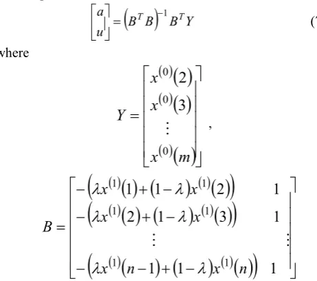
Step 5:aandu in equation (3) can be estimated by using Least Squares Estimation:
B B B Y ua T 1 T
(7) where
m
x
x
x
Y
0 0 03
2
,
1
1
1
1
3
1
2
1
2
1
1
1 1 1 1 1 1n
x
n
x
x
x
x
x
B
Step 6: Based on the estimated coefficientsa and u, the forecasting values of xˆ 0
t
t2,3,,m
can be evaluatedaccording to the following inverse accumulated generating operation (IAGO):
t ma u e a u x t
xˆ1 1 1 at 1 , 2,3,,
(8)
t x
t x
t t mxˆ0 ˆ1 ˆ1 1, 2,3,, (9)
IAENG International Journal of Applied Mathematics, 49:4, IJAM_49_4_25
B. Optimization Principle of the Basic DE
The intelligent optimization algorithm has been proved to be efficient and to quickly reach a quasi-optimal solution with little effort in many fields, such as power systems [25,26], supply chain management [27], portfolio optimization [28], and route optimization [29]. As a typical intelligent algorithm, the DE algorithm, proposed by Storn and Price [30], has been successfully applied to solve problems in many scientific and engineering fields due to its many attractive characteristics, such as compact structure, simple use, fast convergence speed, and robustness. The procedure of the classical DE includes five steps: initialization, evaluation, mutation, crossover, and selection. The details are as follows [31]:
Step 1: Input the population size N, the scaling factor
F[0,2], and the crossover rateCR[0,1]. Then, individuals in the first generation are generated randomly:
0
i1
0, i2 0, , iD
0
i x x x
x
Step 2: For each individualxi(t), evaluate its fitness value
fit(xi(t)).
Step 3: The five most frequently used mutation strategies executed in the basic DE include: "DE/rand/1", "DE/best/1", "DE/rand-to-best/1", "DE/best/2", and "DE/rand/2" [32]. In this paper, since the experiments showed that the above five mutation strategies reach the same optimization accuracy on parameter λ of GM (1,1), the first mutation strategy was adopted:
"DE/rand/1": vxid
t xr1d
t F
xr2d
t xr3d
t
where,d= 1, 2, ..., D. The indicesr1,r2,r3{1, 2, …,N} are mutually exclusive and randomly generated integers, and
r1≠r2≠r3≠i.
Step 4: To increase the diversity of the population, crossover operator is designed: first, an integer
D
drand1,2,, is generated randomly; then, the trail vector uxi
t
uxi1
t,uxi2
t,,uxiD
t
is obtained by thefollowing equation:
D d
t x
d d CR t
v t u
id
rand xid
xid , , 2 , 1
otherwise ,
or 1
, 0 rand if ,
(10)
Step 5: To generate the next generation population, selection operator is implemented by comparing the individuals’ fitness value
otherwise ,
if , 1
t u
t u fit t x fit t
x t
x
xi
xi i
i
i (11)
C. DE-GM
,1,1
modelIn the classical GM (1,1) model, the value of parameter λ defines the prediction performance. In this section, the DE algorithm will be employed to optimize the value of parameter λ, ultimately, to improve the forecasting accuracy of the prediction model.
Table I gives the framework ofDE-GM (1,1, λ) method. In Table I, the Mean Absolute Percentage Error (MAPE) is a stable accuracy measure which was utilized as criterion to evaluate the forecasting performance of a model [33]. PE denotes the percentage error. After using DE to optimize GM (1,1, λ), a best value of λ was obtained, which can minimize the MAPE value. The criteria of MAPE to evaluate the
performance of prediction model are shown in Table II.
TABLE I STEPS OF METHOD 1 Method 1: DE-GM (1,1, λ) method
1. Initialize all parameters of the DE algorithm, and randomly initialize the value ofλwithin region [0,1].
2. Merge the DE algorithm into the GM (1,1, λ) model: Adopting DE in Section III.B to optimize the key parameter λ of GM(1,1, λ) model, and output the best solutionλ*. Where, the fitness function of DE is calculated as follows:
PE
*100%1 1 MAPE
2
m
t
t m
fit
t mt x
t x t x
t ˆ 100%, 2,3, ,
PE 0 0 0
Bring λ* into the GM (1,1, λ) model for data forecasting, and record the prediction value.
TABLE II CRITERIA OF MAPE [34] MAPE (%) Forecasting power
<10 Highly accurate
10-20 Good
20-50 Reasonable
>50 Inaccurate
D. DE-Rolling GM
,1,1
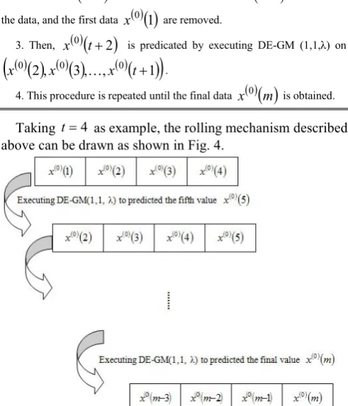
modelIn the classical GM model, the whole data set is used for prediction. In this paper, a rolling mechanism [3] is added to the DE-GM (1,1, λ) model, which is an efficient technique to improve the accuracy of DE-GM (1,1, λ).
TABLE III STEPS OF METHOD 2 Method 2: DE-Rolling GM (1,1, λ) method
1. Executing Method 1 on data series
x0 1,x0 2,,x0 t
(t<m) to predicate x 0
t1 .2. After x 0
t1 is obtained, the new data x 0
t1 are added tothe data, and the first data x 0
1 are removed.3. Then, x 0
t2
is predicated by executing DE-GM (1,1,λ) on
x0 2,x0 3,,x0 t1
.4. This procedure is repeated until the final data x 0
m is obtained. [image:4.595.304.550.472.759.2]Taking t4 as example, the rolling mechanism described above can be drawn as shown in Fig. 4.
Fig. 4. Rolling mechanism of the DE-GM (1,1, λ) model
IAENG International Journal of Applied Mathematics, 49:4, IJAM_49_4_25
Additionally, the fitness function of the DE-Rolling GM (1,1, λ) is evaluated as:
*100%
data ata dˆ data min
Year Year Year
Year
fitness (12)
where, in this paper, the year ranges from 2009 to 2017.
IV. NUMERICAL EVALUATION
The data (see TABLE IV) was obtained from the China Federation of Electric Power Industry Development and Environmental Resources Department and was used to evaluate and test the forecasting performance of the proposed model and to study the trend of electricity consumption and power generation of China.
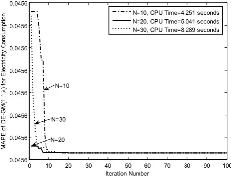
For the DE algorithm, selecting the population size will affect the optimization performance of DE. Computational complexity analysis indicates that the larger the population size, the greater the possibility to identify the global optimal solution. However, the quality of the optimal solution does not always improve with increasing population size. Sometimes, increasing the population size will decrease the accuracy of the optimal solution. To improve the search performance of the algorithm, the performance of DE-GM (1,1,λ) under different population sizes is studied in this paper, and the results are shown in Fig. 5.
0 10 20 30 40 50 60 70 80 90 100
0.0456 0.0456 0.0456 0.0456 0.0456 0.0456 0.0456 0.0456
Iteration Number
M
A
P
E
o
f D
E
-G
M
(1
,1
,
) f
or
E
le
ct
ric
ity
C
on
su
m
pt
io
n N=10, CPU Time=4.251 seconds
N=20, CPU Time=5.041 seconds N=30, CPU Time=8.289 seconds
N=10
N=30
[image:5.595.61.295.365.545.2]N=20
Fig. 5. Performance of DE in Different Population Sizes
Fig. 5 shows that although DE can identify the quasi optimal solution regardless of population sizeN= 10, 20, or 30, whenN= 20, DE has the fastest convergence speed and only requires moderate computing time. To balance the
relationship between the search performance and the calculating time, this paper takes N= 20. Other parameters setting of DE algorithm are selected as: maximum iteration numberTmax= 100; scaling factorF= 2.0; crossover rateCR
= 0.4.
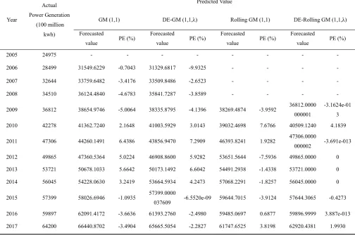
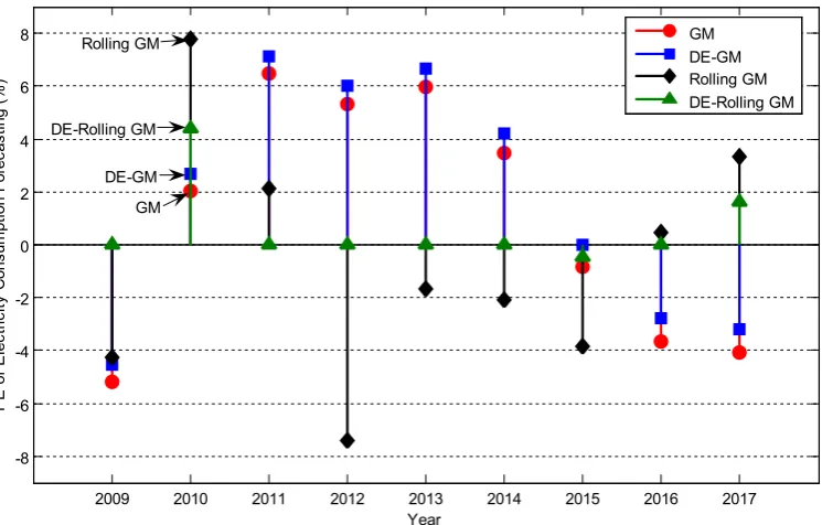
Table IV provides the actual values of electricity consumption and power generation of China (2005-2017). The values in Table IV are from the China Federation of Electric Power Industry Development and Environmental Resources Department.Tables V and VI show the predicted results and the percentage errors of electricity consumption and power generation using four models. Figures 6-9 are drawn based on the data presented in Tables V and VI. Figures 6 and 7 more intuitively and clearly show the gaps between the four prediction models and the actual value. Figures 8 and 9 show percentage errors of the four prediction models for electricity consumption and power generation of China, respectively.
In Table V, the best identified value of λ in the DE-GM (1,1,λ) model is λ*= 0.42419538345853; and the best found
values of λ in DE-Rolling GM (1,1,λ) model are λ*{2009-2017}= {0.15509982605890, 1, 0.65542212937978, 0.08700530662786, 0.34055201367078, 0.23744728766230, 0, 0.63416346198740, 1}. In Table VI, the best identified value of λ in the DE-GM (1,1,λ) model is λ* =
0.40160352224665; and the best identified values of λ in the DE-Rolling GM (1,1,λ) model are λ*{2009-2017} = {0.17785393240218, 1, 0.63695789444329, 0.07532105753939, 0.36121529419271, 0.26699033398297, 0, 0.68773028849322, 1}.
The prediction accuracy is directly related to the prediction performance of the model. Therefore, to further compare the prediction performance of all four prediction models, besides MAPE, the other two precision measurement methods (named mean squared error (MSE) and mean absolute deviation (MAD)) were also used for the accuracy comparison of the four models. MAD and MSE are defined as follows:
mt
t
x
t
x
m
12 0 0
ˆ
1
MSE
(13)
mt
t
x
t
x
m
10 0
ˆ
1
MAD
(14)Based on the data in Tables V and VI, the MAPE, MSE, and MAD of the four models are given in Table VII.
TABLE IV
ACTUAL ELECTRICITY CONSUMPTION AND POWER GENERATION OF CHINA (2005-2017) (100 MILLION KWH)
Year 2005 2006 2007 2008 2009 2010 2011 2012 2013 2014 2015 2016 2017
Electricity
Consumption 24781 28368 32565 34380 36598 41999 47026 49657 53423 55637 56933 59198 63000 Power
Generation 24975 28499 32644 34510 36812 42278 47306 49865 53721 56045 57399 59897 64200 Data sources: “2010 compilation of statistical data of electric power
industry” and “Summary of the statistical data of the power industry (2010-2017)” from the China Federation of Electric Power IndustryDevelopment and Environmental Resources Department.
IAENG International Journal of Applied Mathematics, 49:4, IJAM_49_4_25
TABLE V
FORECASTED VALUES AND ERRORS OF ELECTRICITY CONSUMPTION USING THE FOUR MODELS
Year
Actual Electricity Consumption
(100 million kwh)
Predicted Value
GM (1,1) DE-GM (1,1,λ) Rolling GM (1,1) DE-Rolling GM (1,1,λ)
Forecasted
value PE (%)
Forecasted
value PE (%)
Forecasted
value PE (%)
Forecasted
value PE (%)
2005 24781 - - -
-2006 28368 31529.7859 -11.1456 31362.7956 -10.5569 - -
-2007 32565 33700.1744 -3.4858 33510.9633 -2.9048 - -
-2008 34380 36019.9641 -4.7701 35806.2679 -4.1485 - -
-2009 36598 38499.4391 -5.1954 38258.7874 -4.5379 38155.0801 -4.2545 36597.9999 3.181e-013 2010 41999 41149.5916 2.0224 40879.2901 2.6660 38743.5014 7.7513 40158.5720 4.3820
2011 47026 43982.1704 6.4726 43679.2819 7.1167 46015.1825 2.1494 47026.0000
000001 1.238e-013 2012 49657 47009.7329 5.3311 46671.0568 6.0131 53324.1529 -7.3849 49657.0000 0 2013 53423 50245.7011 5.9474 49867.7507 6.6549 54319.7595 -1.6786 53423.0000 0 2014 55637 53704.4208 3.4735 53283.3993 4.2302 56784.4440 -2.0623 55637.0000 0
2015 56933 57401.2254 -0.8224 56932.9999 5.000e-012 59123.8268 -3.8480 57201.1350 -0.4709
2016 59198 61352.5038 -3.6394 60832.5768 -2.7612 58919.4142 0.4705 59198.0000 0 2017 63000 65575.7729 -4.0885 64999.2518 -3.1734 60915.4460 3.3088 61985.6526 1.6100
TABLE VI
FORECASTING VALUES AND ERRORS OF POWER GENERATION USING THE FOUR MODELS
Year
Actual Power Generation
(100 million kwh)
Predicted Value
GM (1,1) DE-GM (1,1,λ) Rolling GM (1,1) DE-Rolling GM (1,1,λ)
Forecasted
value PE (%)
Forecasted
value PE (%)
Forecasted
value PE (%)
Forecasted
value PE (%)
2005 24975 - - -
-2006 28499 31549.6229 -0.7043 31329.6817 -9.9325 - - -
-2007 32644 33759.6482 -3.4176 33509.8486 -2.6523 - - -
-2008 34510 36124.4840 -4.6783 35841.7287 -3.8589 - - -
-2009 36812 38654.9746 -5.0064 38335.8795 -4.1396 38269.4874 -3.9592 36812.0000 000001
-3.1624e-01 3 2010 42278 41362.7240 2.1648 41003.5929 3.0143 39032.4698 7.6766 40509.1240 4.1839
2011 47306 44260.1491 6.4386 43856.9470 7.2909 46393.8241 1.9282 47306.0000
000002 -3.691e-013 2012 49865 47360.5364 5.0224 46908.8600 5.9282 53651.5644 -7.5936 49865.0000 0 2013 53721 50678.1033 5.6642 50173.1492 6.6042 54491.2938 -1.4338 53721.0000 0
2014 56045 54228.0630 3.2419 53664.5934 4.2473 57068.2291 -1.8257 56045.0000 0
2015 57399 58026.6946 -1.0935 57399.0000
037609 -6.5520e-09 59644.7015 -3.9124 57644.3065 -0.4273 2016 59897 62091.4172 -3.6636 61393.2760 -2.4980 59485.0697 0.6877 59896.9999 3.887e-013 2017 64200 66440.8702 -3.4904 65665.5054 -2.2827 61747.6525 3.8198 62920.4381 1.9930
IAENG International Journal of Applied Mathematics, 49:4, IJAM_49_4_25
TABLE VII
COMPARATIVE ANALYSIS OF FORECASTING ERRORS
Models MAPE (%) MSE MAD
Actual Electricity Consumption
GM (1,1) 4.6995 4.9926e+006 2.0573e+003
DE-GM (1,1,λ) 4.5636 5.0729e+006 2.0019e+003
Rolling GM (1,1) 3.6565 4.3151e+006 1.7876e+003
DE-Rolling GM (1,1,λ) 0.7181 4.9866e+005 346.9901
Power Generation
GM (1,1) 4.5488 4.6444e+006 2.0010e+003
DE-GM (1,1,λ) 4.3707 4.8131e+006 1.9268e+003
Rolling GM (1,1) 3.6486 4.5217e+006 1.8117e+003
DE-Rolling GM (1,1,λ) 0.7338 5.3626e+005 365.9716
20042 2006 2008 2010 2012 2014 2016 2018
2.5 3 3.5 4 4.5 5 5.5 6 6.5
7x 10
4
Year
E
le
ct
ric
ity
C
on
su
m
pt
io
n
of
C
hi
na
(1
00
m
ill
io
n
kw
h)
Actual Electricity Consumption GM
DE-GM Rolling GM DE-Rolling GM
Actual Electricity Consumption
GM
DE-GM Rolling GM
[image:7.595.91.478.486.737.2]DE-Rolling GM
Fig. 6. Comparison of the actual and forecasting electricity consumption curves
20042 2006 2008 2010 2012 2014 2016 2018
2.5 3 3.5 4 4.5 5 5.5 6 6.5
7x 10
4
Year
P
ow
er
G
en
er
at
io
n
of
C
hi
na
(1
00
m
ill
io
n
kw
h)
Actual Power Generation GM
DE-GM Rolling GM DE-Rolling GM
Actual Power Generation
GM
DE-GM Rolling GM
DE-Rolling GM
Fig.7. Comparison of the actual and forecasting power generation curves
IAENG International Journal of Applied Mathematics, 49:4, IJAM_49_4_25
2009 2010 2011 2012 2013 2014 2015 2016 2017 -8
-6 -4 -2 0 2 4 6 8
Year
P
E
o
f E
le
ct
ric
ity
C
on
su
m
pt
io
n
Fo
re
ca
st
in
g
(%
)
GM DE-GM Rolling GM DE-Rolling GM Rolling GM
[image:8.595.103.476.67.305.2]DE-Rolling GM DE-GM GM
Fig. 8. Percentage error graph of electricity consumption forecasting using four models (2009-2017)
2009 2010 2011 2012 2013 2014 2015 2016 2017
-8 -6 -4 -2 0 2 4 6 8
Year
P
E
o
f P
ow
er
G
en
er
at
io
n
Fo
re
ca
st
in
g
(%
)
GM DE-GM Rolling GM DE-Rolling GM Rolling GM
DE-Rolling GM
[image:8.595.98.478.342.584.2]DE-GM GM
Fig. 9. Percentage error graph of power generation forecasting using four models (2009-2017)
Table VII shows that the accuracy of the DE-Rolling GM (1,1,λ) model is outperforms those of the other three models, since the MAPE, MSE, and MAD of DE-Rolling GM (1,1,λ) are the smallest of the four models. Table VII also shows that the accuracy of the DE-GM (1,1,λ) model is higher than that of the classical GM (1,1) model, and the accuracy of DE-Rolling GM (1,1,λ) model is higher than that of the Rolling GM (1,1) model. Therefore, these results indicate that the optimized parameter λ can improve the prediction accuracy. Figures 6 and 7 show that the fitting degree of DE-Rolling GM (1,1,λ) to the actual data is the highest among the four models. Moreover, Figures 8 and 9 indicate more intuitively that the percentage error of the DE-Rolling GM (1,1,λ) is almost the lowest of the four models.
Since the DE-Rolling GM (1,1,λ) model has the highest accuracy among all four models, the DE-Rolling GM (1,1,λ) model was adopted to predict the electricity consumption and power generation of China for the next eight years (2018-2025), and the forecasting results are presented in TABLE VIII.
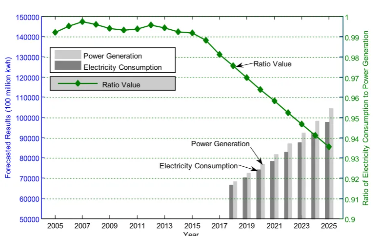
To further explore the electricity utilization, the ratio of electricity consumption to electricity generation was calculated from 2005 to 2025, and the results are shown in Table IX. Based on the data in Tables VIII and IX, the ratio curves of electricity consumption and power generation (2005-2025) and the growth trend of China’s electricity consumption and power generation for the next eight years are presented in Figure 10.
IAENG International Journal of Applied Mathematics, 49:4, IJAM_49_4_25
TABLE VIII
FORECASTING RESULTS (2018-2025) BASED ON DE-ROLLING GM (1,1,λ)
Year
Electricity consumption Power generation
Best found value of parameterλ
Forecasting results (100 million kwh)
Best found value of parameterλ
Forecasting results (100 million kwh)
2018 0.56471315806054 66308.0951 0.56617111016713 67944.0455
2019 0.47911037980164 70156.8678 0.47947685788859 72337.7556
2020 0.51729787243814 74044.3628 0.51782123675458 76798.2998
2021 0.49866820649168 78239.6720 0.49919547247237 81642.6474
2022 0.50739111871292 82626.3249 0.50786461010381 86737.9715
2023 0.50322521945293 87282.1533 0.50374617285558 92178.6666
2024 0.50519632130281 92188.6815 0.50568403352268 97946.9016
[image:9.595.58.545.102.566.2]2025 0.50425954334697 97376.8658 0.50476805316580 104082.9798
TABLE IX
RATIO OF ELECTRICITY CONSUMPTION TO POWER GENERATION
Year 2005 2006 2007 2008 2009 2010 2011 2012 2013 2014 2015 2016 2017
Ratio Value 0.9922 0.9954 0.9976 0.9962 0.9942 0.9934 0.9941 0.9958 0.9945 0.9927 0.9919 0.9883 0.9813
Year 2018 2019 2020 2021 2022 2023 2024 2025
Ratio Value 0.9759 0.9699 0.9641 0.9583 0.9526 0.9469 0.9412 0.9356
2005 2007 2009 2011 2013 2015 2017 2019 2021 2023 2025
50000 60000 70000 80000 90000 100000 110000 120000 130000 140000 150000
Fo
re
ca
st
ed
R
es
ul
ts
(1
00
m
ill
io
n
kw
h)
0.9 0.91 0.92 0.93 0.94 0.95 0.96 0.97 0.98 0.99 1
Year
R
at
io
o
f E
le
ct
ric
ity
C
on
su
m
pt
io
n
to
P
ow
er
G
en
er
at
io
n
Power Generation Electricity Consumption
Ratio Value
Power Generation
Electricity Consumption
[image:9.595.98.489.318.560.2]Ratio Value
Fig. 10. Forecasting curves of electricity consumption and power generation of China (2018-2025) based on DE-Rolling GM (1,1,λ) and ratio of electricity consumption to power generation (2005-2025)
Table VIII shows that the electricity consumption and power generation of China are increasing, showing a steady growth over the next eight years; however, the growth rate of electricity consumption is not as fast as that of power generation after 2012. As intuitively visible from Figure 10, the ratio of electricity consumption to power generation fluctuated from 2005 to 2012, but has been in decline since 2012. Based on the prediction data using DE-Rolling GM (1,1,λ) model, the ratio may decrease to 0.9356 in 2025.
V. CONCLUSION
Affected by many unstable and unpredictable factors in economy and social development, guaranteeing a realistic electricity supply is a great challenge for the power utilities of China and of other countries. Hence, forecasting the
electricity consumption is important for every government. Along with the high-speed growth of industrialization and urbanization in China, the electricity consumption and power generation in China maintains a rapid growth.
This paper constructs a prediction model by using the GM (1,1,λ) model based on rolling mechanism and DE algorithm. This experimental study has demonstrated that the proposed DE-Rolling GM (1,1,λ) model achieves a higher accuracy than three other assessed models, which suggests that adopting this approach for the modeling of China's electricity consumption and power generation is both reliable and efficient. Based on the DE-Rolling GM (1,1,λ) prediction model, considering trends of historical data, the electricity consumption and power generation of China will reach 9737.687 billion kWh and 10408.298 billion kWh, respectively, in 2025. In addition, the results show that the
IAENG International Journal of Applied Mathematics, 49:4, IJAM_49_4_25
ratio of electricity consumption to power generation has decreased since 2012, and this deceleration is accelerating, which indicates that China's power utilization rate is gradually declining. If effective measures will not be taken in the future, China's ratio of electricity consumption to power generation is likely to decrease from 0.9813 in 2017 to 0.9356 by 2025. Therefore, the power sector should pay attention to this trend and initiate corresponding measures (such as slowing down the growth of power generation) to avoid a further decline of the power utilization rate, to save resources. The proposed prediction model provides a basis for electricity supply planning for power departments to ensure the balance of power supply and demand and to improve the utilization rate of electricity.
ACKNOWLEDGMENT
The work was supported by the National Natural Science Foundation of China [71802004, 71801076, 71771003], Natural Science Foundation of Anhui Province [1808085QG231, 1808085QG222, 1808085MG215], Philosophy and Social Science Project of Anhui Province [AHSKY2016D21, AHSKY2016D25].
REFERENCES
[1] Zhou W. Z., He J. M. Generalized GM (1,1) model and its application in forecasting of fuel production. Applied Mathematical Modelling, 2013, 37: 6234-6243. [2] Deng J. L. Gray system theory. Huazhong University of
Science & Technology Press, Wuhan. 1990.
[3] Akay D. Grey prediction with rolling mechanism for electricity demand forecasting of Turkey. Energy, 2007, 32: 1670-1675.
[4] Yuan C., Liu S., Fang Z., Comparison of China's primary energy consumption forecasting by using ARIMA (the autoregressive integrated moving average) model and GM(1,1) model. Energy, 2016, 100: 384-390.
[5] Ding S. A novel self-adapting intelligent grey model for forecasting China's natural-gas demand. Energy, 2018,162: 393-407.
[6] Zeng B., Duan H., Bai Y., Meng W. Forecasting the output of shale gas in China using an unbiased grey model and weakening buffer operator. Energy, 2018, 151: 238-249.
[7] Peng G., Wang H., Song X., Zhang H. Intelligent management of coal stockpiles using improved grey spontaneous combustion forecasting models. Energy, 2017, 132: 269-279.
[8] Li S., Ma X., Yang C. Prediction of spontaneous combustion in the coal stockpile based on an improved metabolic grey model. Process Safety and Environmental Protection, 2018, 116: 564-577. [9] Hao H., Zhang Q., Wang Z., Zhang J. Forecasting the
number of end-of-life vehicles using a hybrid model based on grey model and artificial neural network. Journal of Cleaner Production, 2018, 202: 684-696. [10] Ene S., Öztürk N. Grey modelling based forecasting
system for return flow of end-of-life vehicles. Technological Forecasting and Social Change, 2017,115: 155-166.
[11] Wang Q., Liu L., Wang S., Wang J. Z., Liu M. Predicting Beijing's tertiary industry with an improved grey model. Applied Soft Computing, 2017 (b), 57: 482-494.
[12] Ma X., Liu Z., Wang Y. Application of a novel nonlinear multivariate grey Bernoulli model to predict the tourist income of China. Journal of Computational and Applied Mathematics, 2019, 347:84-94.
[13] Zeng B., Luo C., Liu S., Bai Y., Li C. Development of an optimization method for the GM(1,N) model. Engineering Applications of Artificial Intelligence, 2016, 55: 353-362.
[14] Wei B., Xie N., Hu A. Optimal solution for novel grey polynomial prediction model. Applied Mathematical Modelling, 2018, 62: 717-727.
[15] Li D. C., Chang C. J., Chen C. C., Chen W. C. Forecasting short-term electricity consumption using the adaptive grey-based approach-An Asian case. Omega, 2012, 40: 767-773.
[16] Zhao H., Guo S. An optimized grey model for annual power load forecasting. Energy, 2016, 107: 272-286. [17] Ding S., Hipel K. W., Dang Y. G. Forecasting China's
electricity consumption using a new grey prediction model. Energy, 2018, 149: 314-328.
[18] Wu L., Gao X., Xiao Y., Yang Y., Chen X. Using a novel multi-variable grey model to forecast the electricity consumption of Shandong Province in China. Energy, 2018, 157: 327-335.
[19] Ma W., Zhu X., Wang M. Forecasting iron ore import and consumption of China using grey model optimized by particle swarm optimization algorithm. Resources Policy, 2013, 38: 613-620.
[20] Li C., Qin J., Li J., Hou Q. The accident early warning system for iron and steel enterprises based on combination weighting and Grey Prediction Model GM (1,1). Safety Science, 2016, 89: 19-27.
[21] Pao H. T., Fub H. C., Tseng C. L. Forecasting of CO2 emissions, energy consumption and economic growth in China using an improved grey model. Energy, 2012, 40: 400-409.
[22] Tabaszewski M., Cempel C. Using a set of GM(1,1) models to predict values of diagnostic symptoms. Mechanical Systems & Signal Processing, 2015, 52-53: 416-425.
[23] Wang Z. X., Li Q., Pei L. L. A seasonal GM(1,1) model for forecasting the electricity consumption of the primary economic sectors. Energy, 2018, 154: 522-534. [24] Wen J. C., Wu Y. P., He Y. The study of α in GM(1,1) model. Journal of the Chinese Institute of Engineers, 2000, 23: 583-589.
[25] Chen G., Yi X., Zhang Z., Qiu S. Solving optimal power flow using cuckoo search algorithm with feedback control and local search mechanism. IAENG International Journal of Computer Science, 2019, 46(2): 321-331.
[26] Chen G., Lu Z., Zhang Z., Sun Z. Research on hybrid modified cuckoo search algorithm for optimal reactive power dispatch problem. IAENG International Journal of Computer Science, 2018, 45(2): 328-339.
[27] Wang M., Zhang R. Zhu X. A bi-level programming approach to the decision problems in a vendor-buyer
IAENG International Journal of Applied Mathematics, 49:4, IJAM_49_4_25
eco-friendly supply chain, Computers & Industrial Engineering, 2017, 105: 299-312.
[28] Wang J. A novel firefly algorithm for portfolio optimization problem. IAENG International Journal of Applied Mathematics, 2019, 49(1): 45-50.
[29] Tutuko B., Nurmaini S., Saparudin, Sahayu P. Route optimization of non-holonomic leader-follower control using dynamic particle swarm optimization. IAENG International Journal of Computer Science, 2019, 46(1):1-11.
[30] Storn R., Price K. Differential evolution-a simple and efficient heuristic for global optimization over continuous spaces. Journal of Global Optimization, 1997 , 11 (4) : 341-359.
[31] Price K. V., Storn R. M., Lampinen J. A. Differential evolution: A practical approach to global optimization. Berlin: Springer, 2005.
[32] Zhao S.Z., Suganthan P.N., Das S. Self-adaptive differential evolution with multi-trajectory search for large-scale optimization. Soft Computing, 2011, 15: 2175-2185.
[33] Lee S. C., Shih L. H. Forecasting of electricity costs based on an enhanced gray-based learning model: A case study of renewable energy in Taiwan. Technological Forecasting & Social Change, 2011, 78: 1242-1253.
[34] DeLurgio S. A. Forecasting Principles and Applications. Irwin/ McGraw-Hill, New York, 1998.