Proposal of Fast and Secure Clustering Methods
for IoT
Hirofumi Miyajima, Hiromi Miyajima, and Norio Shiratori
Abstract—Cloud (computing) system has been widely used as one of ICTs. However, as the number of terminals connected to it increases, the limit of the capability is also becoming apparent. The limit of its capability leads to the delay of significant processing time. In order to improve this, the edge (or fog) computing system has been proposed. In the conventional cloud system, a terminal sends all data to the cloud and the cloud returns the computation result to the terminal (or thing) directly connected to it. On the other hand, in the edge (computing) system, a plural of servers called edges are assigned between the cloud and the terminal (or thing). In the system, there are two groups of servers for cloud and edge. Heavy and normal tasks are processed in cloud and edge servers, respectively. Then, let us consider about machine learning in cloud or edge system. The purpose of learning is to find out the relationship (information) lurking in from the collected data. That is, a system with several parameters is assumed and estimated by repeatedly updating the parameters with learning data. Further, there is the problem of the security for learning data. How can we build cloud system to avoid such risk? Secure multiparty computation (SMC) is known as one method realizing secure computation. Many studies on learning methods based on SMC have also been proposed in the cloud system. Then, what kind of learning method is suitable for edge system based on SMC? In this paper, we will propose Neural Gas (NG) algorithms to realize fast and secure processing on edge computing for clustering and classification problems, and show the effectiveness of the proposed methods in numerical simulations.
Index Terms—IoT, Machine learning, Security, Batch learn-ing, Clusterlearn-ing, Classification problem, Neural Gas.
I. INTRODUCTION
C
LOUD (computing) system has been widely used as one of ICTs. The cloud computing is a system where multiple users (clients) use servers with high capability, so it is possible to reduce operating costs. In conventional cloud computing, data management and calculation processing are collectively performed on servers of the cloud. In IoT (Inter-net of Things), however, the number of clients connected to the cloud is very large compared with the traditional system. As a result, it is known that the processing capability may be degraded[1], [2], [3], [4]. In order to improve this, the edge (or fog) computing system has been proposed. In the conventional cloud system, a terminal (or thing) sends all data to the cloud and the cloud returns the computation result to the terminal (or thing) directly connected to it. In the edge system, a plural of servers called edges are connected directly or to close distance between the cloud and the terminal (or thing). That is, although terminals of edge system do not use servers with high processing capability directly, it seems that high processing capability can be realized by efficiently combining a plural servers in the edge system. From theHirofumi Miyajima is Faculty of Informatics, Okayama University of Science, Japan e-mail: [email protected]
Hiromi Miyajima is with Former Kagoshima University. Norio Shiratori is with Chuo University.
side of terminals, normal tasks can be handled at edges, and the cloud processing is used for tasks that require large computing power. Then, what kind of paradigm for machine learning with the edge computing is needed? The purpose of learning is to find out the relationship (information) lurking in from the collected data. In order to realize this, a system with several parameters is assumed and estimated by repeatedly updating the parameters with learning data[7]. Further, users of cloud or edge computing cannot escape the concern about the risk of information leakage. How can we build cloud or edge computing system to avoid such risks and to perform fast learning? One way to achieve this goal is to use data encryption. Data encryption is an effective way to protect data from risk, but data must be repeatedly encrypted and decrypted each time data processing is done. Therefore, a safe system using distributed processing has attracted attention, and a lot of studies with cloud have been proposed[8], [9]. SMC is one of the typical model of them[5], [6]. However, there are little studies about SMC model with IoT. In order to perform it, we showed the effectiveness of batch processing for BP of neural network in the previous paper[12]. In this paper, we will propose NG algorithms to realize fast and secure processing on edge computing for clustering and classification problems, and show the effectiveness of the proposed methods in numerical simulations.
II. PRELIMINARY
A. A configuration of edge computing system
The purpose of the edge system is to perform the effective computation by combining multiple servers with low capabil-ity to build a system with high processing capabilcapabil-ity[1], [2], [3]. Fig.1(a) and (b) show two images for the conventional and edge systems, respectively. In the conventional cloud system, each terminal that needs calculation processing sends all data to the cloud and returns the computation result to the terminal directly connected to the cloud (See Fig.1 (a)). Fig.1(b) is composed of the terminals (or things) directly connected to the cloud and a plural servers (called edges) connected directly or to close distance between the cloud and the terminal (or things). Each server is connected directly to each terminal (or thing). The problem is how to share and distribute data between the client and the server in order to execute fast computation while maintaining security. In this paper, a system shown in Fig.2 is assumed as an example for local servers of edge system.
B. Steepest descent method in machine learning
can not be found directly, parameters are estimated by se-quentially updating the parameters based on SDM (Steepest Descent Method)[7]. Applications of SDM include BP (Back Propagation) learning of neural network, unsupervised learn-ing like K-means and NG (Neural Gas) and fuzzy modellearn-ing, etc.
SDM is a way to minimize an evaluation function T(θ)
parameterized by a system parametersθ∈Rdby updating the parameters in the opposite direction of the gradient ∂T(θ)
∂θ of
the evaluation function to the parameters, whereRis the set of all real numbers. The learning rate η determines the size of the steps we take to reach a (local) minimum. The method is performed based on the following equation[7] :
θ(t+ 1) =θ(t)−η∇T(θ) (1)
That is, the parameterθis updated based on Eq.(1) using learning data in order to reach a minimum. There are three methods based on how to use learning data, online, batch and batch. In the following, let us explain the mini-batch method[7].
LetD be the set of learning data and Zi={1,· · ·, i}for
a positive integer i. The set D is composed of L subsets such asD =∪Ll=1Bl andBi∩Bj = ø for i̸=j∈ZL, where
|Bl|=bl forl∈ZL and|D|=
∑L l=1bl.
Lett= 1. Letεbe a small number.
Learning Algorithm A (Mini-batch learning) Input : The set D of learning data
Output : System parametersθ Step A1 : The set Bl is given.
Step A2 : The parameter θ based on Eq.(1) for Bl is
updated.
Step A3 : If ∇T(θ)> ε, then go to Step 1 with t←t+ 1
else algorithm terminates.
IfL= 1andL=|D|, then the methods are called online and batch ones, respectively.
C. System configuration of secure shared data for SMC
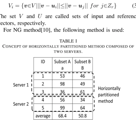
Let us consider about conventional works with secure shared data for SMC. In order to solve the problem, three par-titioned representation of data such as horizontally, vertically and any partitioned methods for SMC are well known[8], [9]. Let us explain about the horizontally partitioned method using an example of Table I. In Table I, a and b are original data (marks) and ID is student identifier. The purpose of computation is to get the average of them.
All the data are shared into two servers, Server 1 and Server 2 as follows:
Server 1: dataset for ID=1, 2, 3, Server 2: dataset for ID=4, 5.
In Server 1, each average for A or B is computed as(53 + 98 + 36)/3 and (46 + 49 + 61)/3, respectively. In Server 2, each average for A or B is computed as (56 + 99)/2
and(34 + 64)/2, respectively. As a result, two averages for subsets A and B are 68.4 and 50.8, respectively. Each server cannot know half of the dataset, so security preserving hold. In the following, secure learning methods are proposed by using horizontally partitioned method.
(a) Conventional system
[image:2.595.356.547.63.313.2](b) Edge system
Fig. 1. Cloud and edge systems.
Fig. 2. An example for local servers of edge system.
D. Neural gas method
Vector quantization techniques encode a data space, e.g., a subspaceV⊆Rd, utilizing only a finite setU ={u
i|i∈Zr}
of reference vectors (also called cluster centers), wheredand
rare positive integers, respectively.
Let the winner vectorui(v)be defined for any vectorv∈V
as follows:
i(v) = arg min
i∈Zr
||v−ui|| (2)
From the finite setU,V is partitioned as follows:
Vi={v∈V|||v−ui||≤||v−uj|| f or j∈Zr} (3)
The set V and U are called sets of input and reference vectors, respectively.
For NG method[10], the following method is used:
TABLE I
[image:2.595.308.544.583.791.2]Given an input vectorv, we determine the neighborhood-ranking uik for k∈Zr∗−1, being the reference vector for
which there are kvectorsuj with
||v−uj||<||v−uik|| (4)
Letα∈[0,1]andλ >0.
If we denote the numberkassociated with each vectorui
byki(v,ui), then the adaption step for adjusting theui’s is
given by
△ui=αhλ(ki(v,ui))(v−ui) (5) hλ(ki(v,ui)) = exp (−ki(v,ui)/λ)) (6)
α=αint
( αf in αint
) t Tmax
where the following function is used as an evaluation one :
E= ∑
ui∈U
∑
v∈V
hλ(ki(v,ui))
∑
ul∈Uhλ(kl(v,ul))
||v−ui(v)||2 (7)
The number λis called decay constant.
If λ→0, Eq.(5) becomes equivalent to the K-means method[10].
Letp(v)be the probability distribution of data vectors for
V. Then, NG method is shown as follows[10] : Learning Algorithm B (Neural Gas)
Input : The set V of input vectors. Output : The set U of reference vectors.
Step B1 : The initial values of reference vectors are set randomly. The learning coefficients αint and αf in are set.
LetTmax be the maximum number of learning time.
Step B2 : Lett= 1.
Step B3 : Give a data v∈V based on p(v) and each neighborhood-rankingki(v,ui)is determined for i∈Zr.
Step B4 : Each reference vector ui for i∈Zr is updated
based on Eq.(5)
Step B5 : Ift≥Tmax, then the algorithm terminates and the
set U ={ui|i∈Zr} of reference vectors for V is obtained
else go to Step B3 as t←t+ 1.
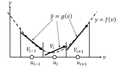
E. Adaptively local linear mapping
The aim in this section is to adaptively approximate the functiony =f(v)withv∈V⊆Rd andy∈R using NG[10].
That is, a supervised learning using NG is introduced. The set V denotes the function’s domain. Let us consider n
computational units, each containing a reference vector ui
together with a constant ai0 and d-dimensional vectors ai.
Learning Algorithm B assigns each uniti to a subregionVi
as defined in Eq.(3), and the coefficients ai0 andai define
a linear mapping
g(v) =ai0+ai(v−ui) (8)
from Rd to R over each of the Voronoi diagram Vi(See
Fig.3). Hence, the function y = f(v) is approximated by
˜
y=g(v) with
g(v) =ai(v)0+ai(v)(v−ui(v)) (9)
wherei(v)denotes uniti with itsui closest tov.
[image:3.595.324.517.55.169.2]To learn the input-output mapping, a series of train-ing steps by givtrain-ing the set of learntrain-ing data D =
Fig. 3. The concept of local linear mapping : The setViis one composed of elementvclosest to the reference vectorui. The intervalViis approximated by a local linear mapping.
{(xp, y
p)|p∈ZP} is performed. In order to obtain the
output coefficients ai0 and ai, the mean squared error
∑
v∈V(f(v)−g(v))
2
between the actual and the obtained output, averaged over subregion Vi, to be minimal is
re-quired for eachi. SDM with respect toai0andaiyields[10]:
△ai0=α′hλ′(ki(v,ui))(y−ai0−ai(v−ui)) (10)
△ai=α′hλ′(ki(v,ui))(y−ai0−ai(v−ui))(v−ui)
(11)
whereα′>0 andλ′ >0.
The method means NG one with the supervised learning. Remark that the case of k-means is included as a special one.
The algorithm is introduced as follows[10] :
Learning Algorithm C (Adaptively approximation using local linear mapping by NG)
Input : Learning data D = {(xp, yp)|p∈ZP} and D∗ =
{xp|p∈ZP}.
Output : The setU of reference vectors and the coefficients
ai0 andai for i∈Zr.
Step C1 : The setU of reference vectors is determined using
D∗by Algorithm B. The subregionVifori∈Zris determined
using U, where Vi is defined by Eq.(3), Vd =∪ri=1Vi and Vi∩Vj = ∅(i̸=j). Let Tmax be the maximum number of
learning time.
Step C2 : Parametersai0andaifori∈Zrare set randomly.
Lett= 1.
Step C3 : A learning data (x, y)∈D is selected based on
p(x). The rankki(x,ui)of xfor the setVi is determined.
Step C4 : Parametersai0andaifori∈Zrare updated based
on Eqs.(10) and (11).
Step C5 : Ift≥Tmax, then the algorithm terminates else go
to Step C3 witht←t+ 1.
III. PROPOSED METHODS OF CLUSTERING AND CLASSIFICATION PROBLEMS FOR EDGE COMPUTING
A. Online unsupervised learning for edge computing
In order to compare the ability of the online method with the batch method, an online learning method will be introduced as one of proposed methods. First, the set D of learning data is divided into m pieces of subsets and each subset Bk is given to the k-th server, whereD =∪mk=1Bk.
The setW of reference vectors is randomly selected and sent it to each server. In Step 1, a constant numberk∗is selected randomly fork∗∈Zmand it is sent to each server. In Step 2,
the task at the k∗-th server is performed. That is, select an elementxrandomly and△wk∗
i is computed based on Eq.(6)
and sent them to Client. In Step 3, each element of the setW
is updated using△wki∗ and the setW is sent to each server. In Step 4, the set W of each server is renewed. In Step 5, check if the maximum number of learning is performed.
The final result of the set W is obtained in Client and each server. The algorithm is shown in Table II.
B. Batch unsupervised learning for edge computing
A batch learning method will be proposed (See Table.III). As the case of online learning, the set D of learning data is divided into m pieces of subsets and each subset Bk is
given to the k-th server. The set W of reference vectors is randomly selected and sent to each server. In Step 1, the update amount△wk
i for each element ofW for k-th server
is computed by adding withx∈Bk and the result is sent to
Client. In Step 2, all update amounts sent from each server are added withk∈Zmand each elementwiofW is updated.
The set W is sent to each server. In Step 3, the set W of each server is renewed. In Step 4, check if the maximum number of learning is performed. The final result of the set
W is obtained in Client. The algorithm is shown in Table III.
C. Batch learning using local linear mapping for edge computing
Let D be the set of learning data. By using the set
D∗ = {xp|p∈Z
P}, the set W of reference vectors is
approximated using Leaning Algorithm B. In each server, the initial parameters of linear mapping for each Voronoi region defined by the sets D and W are set randomly. A batch learning using local linear mapping is proposed shown in Table IV. Likewise, an online learning method is proposed. In Step 1, the rank ki(x,wi) of input x and vector wi
for set W is calculated in each server. By using the result, update amounts △ak
i0 and △aki for the constant aki0 and
the coefficient ak
i of local linear function are computed,
respectively, and they are added with x∈Bk. In Step 2,
update amounts△ai0and△aiare computed by adding with k∈Zm and parameters ai0 and ai for i∈Zr are updated,
respectively. The results are sent to each server. In Step 3, the learning errorEk(t)forBkis computed by using updated
local linear functions and the result is sent to Client. In Step 4, the learning errorE(t)forBis computed by addingEk(t)
withk∈Zm. Further, ifE(t)is smaller than the thresholdθ
or t is larger than the maximum number Tmax of learning
time, then the algorithm terminates else go to Step 1 with
t←t+ 1.
IV. NUMERICALSIMULATIONS
A. Clustering problems
Four real world datasets including Iris, Wine Sonar and BCW data coming from UCI machine learning repository have been considered in this simulation as shown in Table V[13], where#data,#input and#class mean the numbers of data, input variables and classes, respectively. As the initial condition, initial values of W are selected randomly from[0,1]and the maximum number of learning times are
100×#data. Let εint = 0.1 andεf in = 0.01. The problem
is how each dataset is approximately by reference vectors. Tables VI and VII show the results of the misclassification rates, where the misclassification rate means the ratio of the misclassification data to all data, and each result is the average value from twenty trials. Conventional online and batch, and Proposed online and batch mean the conventional online and batch learning methods, and the proposed online and batch learning methods, respectively.
Both results show that approximation accuracy for con-ventional and the proposed methods are almost the same. Therefore, the proposed method has good accuracy and security preserving. Since it is difficult to evaluate direct computing time, the time required for parameter updating of one time for learning data is estimated. In online processing, let O1(1) and O2(1) be the computing time of the error and the time to update parameters for each data of the server, respectively. Then, time complexity of the case is
L(O1(1)+O2(1)). That is, the total time complexity isO(L). On the other hand, in batch processing, when the computing time of parameter updating for (L/m) pieces of learning data is assumed to be O3(L/m), the computing time for all learning data is O(1·O3(L/m)), because all computing for edge server is done at a time. The time complexity is O(O4(m) + 1·O3(L/m)), assuming that the computing
time required for updating at the client isO4(m) by using
the update amount of each server. In this case, since the first term is smaller than the second term, O(O4(m) + 1·O3(L/m))≈O(1·O3(L/m))is estimated. As a result, the speedup ofmtimes in batch processing is expected.
B. Classification problems
In this simulations, 5-fold cross validation as an evaluation method is used: In 5-fold cross validation, all data are randomly partitioned into 5 equal size subsets. Of the 5 subsets, a single subset is kept as data for testing the model, and the remaining 4 subsets are used as training data. The cross validation process is repeated 5 times (the folds) with each of 5 subsets used exactly once as the validation (test) data. The five results from the folds can then be averaged to produce a single estimation.
Tables VIII and IX show the results of comparison be-tween the conventional and the proposed methods. In each box of Tables VIII and IX, Training and Test mean the rate (%) of misclassified data for training and test, respectively. Each value is average from five trials. Further, LLM means local linear mapping.
TABLE II
AN ONLINE UNSUPERVISED LEARNING FOR EDGE COMPUTING OFSMC
Client (Server 0) k-th Edge (Server)
Initial The setW of reference vector is selected randomly and The subsetBkof learning data whereD=∪mk=1Bk condition sent to each server, whereW={wi|i∈Zr}
α,Tmaxandθare given. Sett= 1.
Step 1 Select a server numberk∗and send it to each server.
Step 2 Ifk=k∗, then select a datax∈Bkand calculate
△wk∗
i =ε·hλ(ki(x,wi))·(x−wi)fori∈Zr, wherehλ(ki(x,wi)) = exp(−ki(x,wi)/λ) and send them to Client.
Step 3 Calculatewi←wi+α△wk ∗
i fori∈Zr and send them to each server.
Step 4 Update the setW.
Step 5 Ift≥Tmaxthen the algorithm
terminates else go to Step 1 witht←t+ 1
TABLE III
ABATCH UNSUPERVISED LEARNING FOR EDGE COMPUTING OFSMC
Client (Server 0) k-th Edge (Server)
Initial α,Tmaxandθare given. Sett= 1. The subsetBkof learning data whereD=∪mk=1Bk condition
Step 1 Calculate△wk
i = ∑
x∈Bkε·hλ(ki(x,wi))·(x−wi)
fori∈Zm, where
hλ(ki(x,wi)) = exp(−ki(x,wi)/λ)fori∈Zr and send them to Client.
Step 2 Calculatewi←wi+α ∑m
k=1△w k i for
i∈Zrand send them to each server.
Step 3 Update the weightW.
Step 4 Ift≥Tmaxthen the algorithm
terminates else go to Step 1 witht←t+ 1
TABLE IV
LEARNING METHOD USING LOCAL LINEAR MAPPING
Client (Server 0) k-th Edge
Initial The setW is selected The setBkis given. condition randomly and sent it to servers, Parametersak
i0andaki are set whereW={wi|i∈Zr}. randomly. Lett←1.
α,Tmaxandθare given. Sett←1.
Step 1 Calculateei(x,wi)forx∈Bkandi∈Zr. Calculate△ak
i0= ∑
x∈Bkα
′h
λ′(ki(v,ui))(y−ai0−ai(v−ui))
△aki =∑x∈B
kα
′h
λ′(ki(v,ui))(y−ai0−ai(v−ui))(v−ui) whereα′>0andλ′>0and send to client.
Step 2 Calculate
△ai0←ai0+α ∑m
k=1△a k i0 ai←ai+α
∑m k=1△a
k i fori∈Zrand send them to each server.
Step 3 CalculateEk(t) = ∑
x∈Bk(g(x)−d(x))
2and send them to Client.
Step 4 ComputeE(t) =∑mk=1Ek(t). IfE < θort≥Tmax, then the algorithm terminates else go to Step 1 with
t←t+ 1.
TABLE V
THE DATASET FOR PATTERN CLASSIFICATION
Iris Wine Sonar BCW
#data 150 178 208 683
#input 4 13 60 9
#class 3 3 2 2
and security preserving. In this case, the speedup ofmtimes in batch method is also expected.
V. CONCLUSION
In this paper, secure and fast learning methods for clus-tering and classification problems of IoT were proposed
TABLE VI
CONVENTIONAL AND PROPOSED K-MEANS
Iris Wine Sonar BCW Conventional Error 9.9 8.4 44.9 3.9 online M SE 0.022971 0.142272 1.355330 0.284203 Proposed Error 9.9 9.6 45.0 3.9 online M SE 0.022958 0.144359 1.356710 0.284399 Conventional Error 8.4 6.2 45.7 3.9 batch M SE 0.021869 0.139570 1.350222 0.282916 Proposed Error 5.5 6.6 45.6 3.9 batch M SE 0.019845 0.139581 1.349611 0.282916
TABLE VII
CONVENTIONAL AND PROPOSEDNG
Iris Wine Sonar BCW Conventional Error 4.0 6.8 45.1 3.5 online M SE 0.018999 0.140449 1.358412 0.287604 Proposed Error 4.0 6.8 45.0 3.5 online M SE 0.019068 0.140516 1.357611 0.287342 Conventional Error 4.0 6.6 45.2 3.5 batch M SE 0.018935 0.139837 1.350679 0.286089 Proposed Error 4.0 6.9 45.2 3.5 batch M SE 0.018935 0.139849 1.350689 0.286089
TABLE VIII
CONVENTIONAL AND PROPOSED K-MEANS(LLM)
Iris Wine Sonar BCW Conventional Training 3.7 2.5 0.2 2.8 online Test 4.0 5.1 25.0 3.7 Proposed Training 3.6 2.3 0.3 2.8 online Test 3.9 5.3 25.1 3.5 Conventional Training 3.6 2.5 1.3 2.9 batch Test 3.8 4.8 24.6 3.6 Proposed Training 3.3 2.4 2.1 2.9 batch Test 3.6 4.5 26.7 3.6
TABLE IX
CONVENTIONAL AND PROPOSEDNG (LLM)
Iris Wine Sonar BCW Conventional Training 4.0 2.5 0.2 3.0 online Test 4.0 4.6 25.5 3.5 Proposed Training 3.9 2.6 0,3 2.9 online Test 4.0 4.6 25.4 3.5 Conventional Training 4.0 2.4 0.4 2.9 batch Test 4.0 4.6 25.2 3.4 Proposed Training 3.9 2.4 4.3 2.8 batch Test 3.9 4.6 24.9 3.1
verification in implementation is a future work.
REFERENCES
[1] A. Al-Fuqaha, M. Guizani, M. Mohammadi, M. Aledhari and M. Ayyash, ”Internet of Things : A Survey on Enabling Technologies, Pro-tocols, and Applications”, IEEE Communication Surveys&Tutorials, Vol.17, No.4, pp.2347-2376, 2015.
[2] S. Kitagami, T. Suganuma, T. Ogino and N. Shiratori, ”Proposal of a Multi-agent Based Flexible IoT Edge Computing Architecture Harmonizing Its Control with Cloud Computing”, The Fifth Interna-tional Symposium on Computing and Networking (CANDAR2017), November, 2017.
[3] M. Abdelshkour, ”IoT, from Cloud to Fog Computing”, http://blogs.cisco.com/perspectives/iot-from-cloud-to-fog-computing, Mar.2015 (accessed 18 Jun.2017).
[4] P. G. Lopez, A. Montresor, D. Epema, A, Datta, T. Higashino, A. Iamnitchi, M. Barcellos, P. Felber and E. Riviere, ”Edge-centric Computing : Vision and Challenges”, ACM SIGCOMM Computer Communication Review, Vol.45, Issue 5, pp.37-42, Oct.2015. [5] A. Shamir, ”How to share a secret”, Communications of the ACM,
Vol.22, Issue 11, pp.612-613, 1979.
[6] C. C. Aggarwal, and P. S. Yu, ”Privacy-Preserving Data Mining: Models and Algorithms”, ISBN 978-0-387-70991-8, Springer-Verlag, 2009.
[7] S. Ruder, ”An Overview of Gradient Descent Optimization Algo-rithms”, http://ruder.io/optimizing-gradient-descent/, 2016 (accessed 14 Mar. 2018).
[8] S. Subashini, et al., ”A survey on security issues in service delivery models of cloud computing”, J. Network and Computer Applications, Vol.34,pp.1-11, 2011.
[9] H. Miyajima, N. Shigei, H. Miyajima, Y. Miyanishi, S. Kitagami and N. Shiratori, ”New Privacy Preserving Back Propagation Learning for Secure Multiparty Computation”, Journal of Computer Science,
Vol.43,No.3,pp.270-276, 2016.
[10] T. M. Martinetz, S. G. Berkovich and K. J. Schulten, Neural Gas Network for Vector Quantization and its Application to Time-series Prediction, IEEE Trans. Neural Network, 4, 4, pp.558-569, 1993. [11] H. Miyajima, N. Shigei, H. Miyajima, Y. Miyanishi, S. Kitagami
and N. Shiratori, ”New Privacy Preserving Clustering Methods for Se-cure Multiparty Computation”, Artificial Intelligence Research,Vol.6,
No.1,pp.27-36, 2017.
[12] H. Miyajima, H. Miyajima and N. Shiratori, ”Proposal of Security Preserving Machine Learning of IoT”, Artificial Intelligence Research,
Vol.7,No.2,pp.26-33, 2018.