Abstract—This paper introduces a model for finding the optimal replacement policy for Condition Based Maintenance (CBM) of a system when the information obtained from the gathered data does not reveal the system's exact degradation state, and the process of collecting data is costly or non-costly. The proposed model uses the Proportional Hazards Model (PHM) introduced by D. R. Cox to represent the system’s failure rate. The PHM takes into consideration the system's degradation state as well as its age. Since the acquired information is imperfect, the degradation state of the system is not precisely known. Bayes' rule is used to estimate the probability of being in any of the possible states. The system's degradation process follows a Hidden Markov Model (HMM). By using dynamic programming, the system's optimal replacement policy and its long-run average operating cost are found. Based on the total long-run average cost, the optimal interval between data collection, and the corresponding replacement criterion are specified. A numerical example compares between two systems, one which collects data at no cost, and the other having costly observations. The optimal intervals for data collection and the optimal costs are found in both cases.
Index Terms— Condition Based Maintenance (CBM), Costly Observations, Imperfect Information, Proportional Hazard Model (PHM), Hidden Markov Model (HMM).
I. INTRODUCTION
For a system subjected to Condition Based Maintenance (CBM) program, inspections are performed to obtain proper information about the degradation state of the system. In this paper, the information acquired during the inspections does not reveal the exact degradation state of the system but represents some data which are stochastically related to the system's degradation state [11], [13]. This information is called imperfect or partial. The data are then used to calculate the probability of being in a certain degradation state, and to find the optimal replacement policy. In CBM studies, several models have been used to take into account the system's
Manuscript received May 10, 2008.
Alireza Ghasemi is a PhD. candidate (Department of Industrial Engineering and Mathematics, École Polytechnique of Montréal, C. P. 6079, succursale Centre-ville, Montréal, Québec, Canada, H3C 3A7. e-mail: [email protected]).
Dr. Soumaya Yacout is with the Department of Industrial Engineering and Mathematics, École Polytechnique of Montréal (e-mail: [email protected]).
degradation state. One of these models is the Proportional Hazards Model (PHM), introduced by [4], which has been widely used in medical studies. Recently, an increasing application of the PHM to the CBM is reported [10], [1]. According to the PHM, the system's failure rate (also called hazard rate) is estimated based on its age as well as its degradation state. In this paper, the PHM is used to calculate the optimal replacement policy and long-run average cost for a system with imperfect information.
Afterwards, the unrealistic assumption of non-costly observations is relaxed and the corresponding optimal replacement policy and total long-run average cost are found. In the CBM modeling, if the observations are taken at no cost, the optimal observation interval is zero i.e. the best choice is to monitor the system continuously. That is because the higher frequency of observations will provide more frequent information about the degradation state of the system with no extra cost. Consequently, this will reduce the likelihood of performing unnecessary preventive replacements, hence, will result in a more cost effective maintenance system. When there is considerable cost for collecting and analyzing the observations, an optimal observation interval that minimizes the total maintenance cost including the observations cost should be applied. In reality, in many cases, observations require personnel, equipment, and may be destructive tests, and sometimes it is necessary to stop or suspend the operations when collecting the observations [9]. In addition, some actions for analysis and extraction of useful information may be needed; therefore, some costs are associated to the collection and analysis of observations. Finding the optimal total long-run average cost of the maintenance policy, with costly observations, leads to comparison and selection of the optimal observation interval amongst several possible intervals. The replacement criterion that corresponds to the optimal total long-run average cost is then obtained.
This paper consists of four more sections. In section 2 a brief literature review of the principle models in replacement optimization is presented. Section 3 deals with the assumptions, the details of the proposed model and the optimal solution. Section 4 presents a numerical example. The conclusion and the areas of further researches are presented in section 5.
II. LITERATURE REVIEW
Reference [9] investigated the maintenance policy for a system whose exact degradation state is known through the
Optimal Stategies for non-costly and costly observations in
Condition Based Maintenance
criteria and observation interval that minimizes the long-run average cost of the whole maintenance system. Reference [3] considered a system with perfect information which reveals exactly the system's degradation state. The objective is to determine the next observation schedule, based on the information obtained to date. Reference [7] modeled a CBM policy where both the replacement threshold and the observation schedule are decision variables. It is allowed to have unequal observation periods. Reference [8] considered a system revealing perfect information with an obvious failure which is detected as soon as it happens. Reference [2] considered an optimal observation time with a hidden failure being detected through observation. A pre-defined threshold for the failure is assumed and associated costs are considered for the observations, repairs and replacements. [12] considered a replacement problem for a system with perfect information using PHM while the observations are non-costly.
III. PROBLEM FORMULATION
[image:2.612.78.266.556.658.2]This paper presents optimal replacement policy and optimal inspection interval of a deteriorating system subjected to random failure. The degradation state of the system is represented by a finite set of non-negative integers, i.e. by state space
S
=
{
1, 2,,...,
N
}
. State 1 indicates the best possible state for the system which means that the system is new or like new. The degradation state process{
X t
( )
=
1, 2,...,
N
}
, is a discrete time homogeneous Markov chain withN
unobservable states. AllN
degradation states are working states and do not include the failure state which is a non-working state. Figure 1 shows the Markov transition process between degradation states along with transition from each degradation state to the failure state.p
ij is the probability of going from degradation statei
to the degradation statej
during one observation period knowing that the system has not failed yet, despite the fact that,f
i is the probability of going from degradation statei
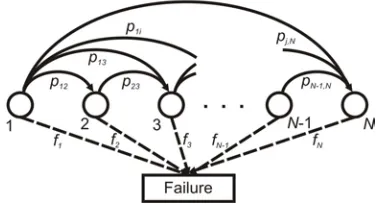
to the failure state. The circles represent the states.Figure 1: Markov process transition and transition to failure The degradation states of the system are not observable except at the time
t
=
0
when the degradation state of the system is certainly 1. The transition matrixP
is an upper triangular matrix, i.e.p
ij=
0
for allj
<
i
, andp
ij=
(
)
( )
(
)
Pr
X t
+ ∆ =
j X t
|
=
i T t
,
> + ∆
,t
= ∆ ∆
0, , 2 ,...
otherwise, meaning that the system degradation state does not improve spontaneously, which is true in most practical cases.T
is a random variable representing the system's failure time. The system indicators are observed at times;, 2 ,...
t
= ∆ ∆
. The indicators obtained,θ
, can take a value ina finite set of
M
non-negative integers, i.e.θ
∈Θ =
{
1, 2,...,
M
}
. It is supposed that a value ofθ
is observed with a known probability ofq
jθ, when the degradation state of the system isj
.Q
represents the stochastic matrix which specifies these probabilities, i.e. Q=
qjθ
, j S∈ ,θ
∈ Θ. The failure is not a degradation state. It is a condition that causes the system to cease functioning and is outwardly obvious. If the failure happens, it is immediately recognized and the only possible action is “Failure Replacement”. Otherwise, at any observation point, we can decide whether to perform “Preventive Replacement” or “Do-Nothing”. Failure Replacement and Preventive Replacement renew the system and return it to state 1 and period k =0. The cost for preventive replacement isC
, while a failure replacement costsK C
+
,K C
,
>
0
. Failure Replacement and Preventive Replacement actions are assumed instantaneous.The system's failure rate is following the PHM. In the PHM, the failure rate of the system
h t X
(
,
k)
=
( ) ( )
0 k
h t
ψ
X
is a product of two independent functions, whereh
0()
.
is a function of the system's age only, andψ
()
.
is a function of the system's degradation state only.( )
kX
=
X k
∆
is the degradation state of the system at periodk
, and∆
is the fixed observation interval. We assume that degradation state of the system remains unchanged during each period, and each degradation state transfer is assumed to take place at the end of each period, just before observation point.The first objective of this work is to determine the optimal replacement policy for the assumed system, while the observation interval is pre-defined and fixed. The second objective is to find the optimal observation interval that minimizes the total long-run average cost per unit time for the replacement and consequently the optimal replacement policy. In the second objective, a considerable cost is assumed for performing the observations.
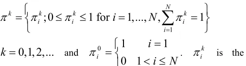
A. Alternative state space
1
;0
1 for
1,..., ,
N1
k k k k
i i i
i
i
N
π
π
π
π
=
=
≤
≤
=
=
∑
0,1, 2,...
k
=
and
≤
<
=
=
N
i
i
i1
0
1
1
0
π
.π
ik is theprobability of being in degradation state
i
atk
th observation point.B. Alternative state's transition
At the
k
+1st observation point, after observingθ
, the prior conditional distribution of the system’s degradation statek
π
, is updated toπ
kj+1( )
θ
which is calculated by using the Bayes’ formula as:( )
1 1
1 1
for
1,...,
N k i ij j
k i
j N N
k i il l i l
p q
j
N
p q
θ
θ
π
π
θ
π
+ =
= =
=
∑
=
∑∑
(1’)This updated conditional distribution carries all the history of the observations and the performed actions since the last replacement. At any replacement, the observation period’s counter
k
, will be reset to 0 and the conditional probability distribution of the system degradation state will be set toπ
0.C. Decision space
The decision space of the model is
{ }
0,∞ , where0
means “Replace the system immediately”, and∞
means “Do-Nothing until the next observation point, or replace at the failure time, if the failure happened before the next observation point”.IV. OPTIMAL REPLACEMENT WITH PRE-DEFINED OBSERVATION INTERVAL
In this section, we assume that the observation interval is pre-set based on the experts' opinion or system’s limitations and will find the optimal replacement policy for the system with the properties assumed earlier.
A. Dynamic Programming Formulation
Let
V
(
k
,
π
k)
denote the minimum cost from periodk
until next renewal point, where the updated conditional distribution of the system degradation state isπ
k:(
, k)
min{
(
0, 0) (
, , k,)
}
V k
π
= C V+π
W kπ
g (1)where C V+
( )
0,π
0 is the expected cost in the case of preventive replacement andW
(
k
,
π
k,
g
)
is the expected cost of leaving the system to work until the next observation point.(
)
(
)
(
)
(
)
( )
(
) (
) (
)
0 1 1
, ,
0, 1 , , , ,
1, Pr | , , ,
k
k k
M
k k k
W k g
K C V R k g k
V k k R k
θ
π
π
π
τ
π
π
+θ
θ
π
π
=
=
+ + − ∆ − ∆
+ + ∆
∑
(2)
(
,
k,
)
R k
π
∆
andτ
(
k
,
π
k,
∆
)
are respectively the probability that the system is still working during thek
+
1st period and, the mean sojourn time of the system duringk
+
1st period when the conditional probability distribution of the system’s degradation state at thek
th period isπ
k, and arecalculated as:
(
)
(
(
)
)
(
)
k i Ni k
k t T k t T k k Rk i t
k
R π π
∑
π=
= ∆
> + ∆ > =
1 , , ,
, |
Pr , ,
(
, ,)
0(
| ,)
(
, ,)
0(
, ,)
a a
k k k k
k a tF dt k dt aR k a R k t dt
τ π =
∫
π + π =∫
πand
(
)
(
)
0
, k, , k,
k R k t dt
τ
π
∆ =∫
∆π
.The failure rate of the system is assumed to follow the PHM, accordingly, the conditional reliability of the system at
k
-th observation point while the degradation state of the system isk
X
is [12]:(
)
( )
(
0 1)
2( ,
, )
|
,
,
,...,
exp
( ) ) ,
k k
k t k k
R k X t
P T
k
t T
k
X X
X
X
h s ds
t
ψ
∆+∆
=
> ∆ +
> ∆
=
−
∫
≤ ∆
[image:3.612.48.301.50.118.2]g
is the average cost of the maintenance policy per unit time over an infinite horizon and consequentlyg
τ
(
k
,
π
k,
∆
)
is the expected cost of the overlapped time of two consecutive replacements of the system when the system has failed and replaced. Figure 2 shows an instance of the case.Figure 2-Observations after a failure replacement
It should be noticed that even after a failure replacement the observations are performed based on the schedule plan.
1 1
Pr( | k) N N k i ij j i j
p qθ
θ π
π
= =
=
∑∑
is probability of observing indicatorθ
atk
+
1st observation epoch knowing that the conditional probability distribution of the system’s degradation state at thek
th period isπ
k.B. Optimal Policy
function of the observed indicator, the age of the system, and
g
, the long-run average cost of the system’s replacement. The decision criterion and the minimum long-run average cost of the system together give the optimum decision criterion for the introduced problem.To continue we adapt the following theorem proved by [6]: Theorem: Assuming that assumptions 1 through 5 as stated in [12] are satisfied, function
V
introduced by equation (1), defined onS
, whereS
is the set of all possible variations of the pair(
k
,
π
k)
, with a constantg
≥
0
, is a bounded measurable non-decreasing function.From equation (2) we can write:
(
)
(
)
(
)
(
)
( )
(
) (
)
(
)
(
)
0
1 0
1
, , 0,
1 , , , ,
1, Pr | , 0,
, ,
k
k k
M
k k
k
W k g C V
K R k g k
V k k C V
R k
θ
π π
π τ π
π θ θ π π
π
+ =
− − =
− ∆ − ∆
+ + − −
∆
×
∑
(3)
Considering that V k
(
+1,π
k+1)
is the minimum expectedreplacement cycle cost at the
k
+
1st period,(
1)
(
0)
1, k 0,
V k+ π + < +C V π
. Since
(
0)
0,
C V+ π is a constant term, by multiplying Pr
(
| , k)
k
θ
π
and summation on all possible observations, it can be shown that:(
1) (
)
(
0) (
)
1
1, Pr | , 0, , , 0
M
k k k
V k k C V R k
θ
π + θ π π π
=
+ − − ∆ <
∑
(4) From (3) and (4) it can be concluded that that if
(
)
(
)
1 , k, , k,
K
−R kπ
∆ <
gτ
kπ
∆ then W k(
,π
k,g)
<
(
0, 0)
C V+
π
so that
V k
(
,
π
k)
=
W k
(
,
π
k,
g
)
. In other words, the optimal action is “Do-Nothing”.
In what follows, assuming that K
1−R k(
,π
k,∆ ≥)
(
, k,)
g
τ
kπ
∆ and at the same time, supposing that the optimal action is “Do-Nothing”, we will show that there is a contradiction. If the statement was true, then from equation (1):(
)
(
)
(
0)
, k , k, 0,
V k π =W k π g < +C V π (5)
From (2) and (5) it can be concluded that:
(
) (
)
(
)
(
)
(
)
(
0)
(
)
1 2
1, ,
1 , , , ,
1, 0, 1 , ,
k k
k k
k k
V k V k
K R k g k
V k C V R k
π π
π τ π
π π π
+ − =
− − ∆ + ∆
+ + − − − ∆
14444244443 1442443
(
)
(
( )
) (
)
(
)
1 1
3
4
1, 1, Pr | ,
, ,
M
k k k
k
V k V k k
R k
θ
π π θ θ π
π
+
=
+ + − +
× ∆
144444444
∑
42444444444
3
14243
(6) Terms 1 and 3 are less than or equal to zero, because of the
definition of
(
1, k)
V k+
π
and considering that it is proved non-decreasing by the theorem. Terms 2 and 4 are bigger or equal to zero by definition. So:(
1, k) (
, k)
0V k+
π
−V kπ
< (6’)On the other hand, since
V
(
k
,
π
k)
is non-decreasing in(
k
,
π
k)
, then V k(
+1,π
k) (
−V k,π
k)
≥0, which is a contradiction to (6’), so equation (5) is not true and
(
0)
(
)
0, , k,
C V+
π
<W kπ
g . This means that the optimal action is “Preventive Replacement”. The whole replacement policy can be expressed by the optimal stopping time *g
T
as:(
)
(
)
{
}
*
*
.inf 0 : 1 , k, , k,
g
T = ∆ k ≥ K
−R kπ
∆ ≥
gτ
kπ
∆(7) In other words, the optimal decision a k
(
,π
k)
at observationpoint
k
with conditional probability distribution of degradation stateπ
kis:(
)
1(
(
, ,)
)
**(
(
, ,)
)
1 , , , ,
if ,
0 if
k k
k k
k K R k g k
K R k g k
a k π τ π
π τ π
π
− ∆ < ∆− ∆ ≥ ∆
∞
=
(8) It can be noticed that the optimal policy is a function of
g
*,the optimum long-run average cost. Next section presents the formulation leading to the calculation of
g
*.C. Optimal long-run average cost
Reference [5] found the long-run average cost per unit of time:
(
)
(
)
min
Pr
,
g g
T
g
C K
T
T
E
T T
φ
=
+
>
(9)where
T
g is stopping-time,T
is the time to failure,Pr(
T
g>
T
)
is the probability of a failure replacement, and min( , )
gwhere g* =minφTg, minimizes
φ
Tg and the value ofg
* is the unique solution ofg
=
φ
Tg.To calculate
E
min( , )
T T
g , we defineW j
(
,
π
j)
as:(
,
j)
W j
π
=
{
min
(
,
)
| ,
(
j)
}
gE
T T
− ∆
j
j
π
(10)It indicates the residual time to replacement at period
j
i.e. the average remaining life fromj
∆
to failure, when the conditional probability distribution of the system’s degradation state isπ
j, and a giveng
, that forces the system to haveT
g that satisfies equation (7) (see Figure 3). Also consider :( )
gt
π
=
(
)
(
)
{
|
r R
+K
1
R r
, ,
π
g r
τ
, ,
π
}
∆
∈
−
∆ =
∆
(11)which calculates the real-time of satisfaction of the cost condition in equation (7), for a given cost
g
, at a certain conditional probability distribution of the system’s degradation state,π
. To calculateW
( )
j
,
π
j , we considerk
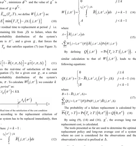
“the hazardous period” as: [image:5.612.108.564.55.544.2](
k
−
1
)
∆ ≤
t
g( )
π
j< ∆
k
Figure 3-Real time of the satisfaction of the cost condition
If
j
≥
k
, according to the replacement criterion of equation (7), the system has to be replaced immediately, then(
j
,
j)
=
0
W
π
.In the case where
j
=
k
−
1
:(
)
(
)
0
,
j,
j,
j g
t j
W j
R j
s ds
π
π
π
− ∆
=
∫
(12)And finally, if
j
<
k
−
1
, by conditioning the length of the replacement cycle on the failure time, we showed that:(
)
(
)
( )
(
) (
) (
)
0 1 1
,
,
,
1,
,
,
Pr
| ,
j j
M
j j j
W j
R j
s ds
W j
R j
j
θ
π
π
π
θ
π
θ
π
∆
+
=
=
+
+
∆
∫
∑
(13)
The expected minimum replacement cycle time can then be calculated by:
(
)
{
(
)
(
0)
}
(
0)
min T Tg,
min
T T, g|
0, W 0,E
=
E
π
=
π
(14)(
,
j)
W j
π
is briefly shown in following equation:(
)
(
)
0
0
,
,
,
1
1
j j
j g
t j
j k
W j
R j
s ds
j k
A
j k
π
π
π
− ∆
≥
=
= −
< −
∫
(14)where
(
)
( )
(
) (
) (
)
0
1 1
, ,
1, , , Pr | ,
j
M
j j j
A R j s ds
W j R j j
θ
π
π θ π θ π
∆
+ =
=
+ + ∆
∫
∑
(15)
By defining
Q j
(
,
π
j)
=
Pr
(
T
g≥
T
| ,
(
j
π
j)
)
, a similar calculation to that ofW j
(
,
π
j)
, leads to the following equations:( )
0
( ,
)
1
( ,
,
)
1
1
j j j
g
j k
Q j
R j
t
j
j k
B
j k
π
π
π
≥
= −
− ∆
= −
< −
(16)
where
( )
11
1 ( , , )
( 1, ) Pr( | , ) ( , , )
j
M
j j j
B R j
Q j j R j
θ
π
π + θ θ π π
=
= − ∆ +
+ ∆
∑
(17)The probability of a failure replacement is calculated by:
(
)
(
(
0)
)
(
0)
Pr
T
g>
T
=
Pr
T
g≥
T
| 0,
π
=
Q
0,
π
(18) By using (9), (14) and (16),g
*, the average long run replacement cost, is calculated.The tools presented so far are used to determine the optimal replacement policy and long-run average cost of a system where no cost is considered for the observations and the observation's interval is prefixed at
∆
.V. OPTIMAL OBSERVATION INTERVAL WITH COSTLY OBSERVATIONS
Under the assumption of negligible observation's cost, the selection of observation interval is usually performed based on the experts' opinion. Higher frequency of observations will provide more frequent information on hand, and consequently a better decision can be made. Shorter observation interval decreases the likelihood of unnecessary preventive replacements.
find the optimal replacement policy and optimal observation interval for the system with previously mentioned assumptions.
A. Dynamic Programming Formulation
We assume that each observation costs
C
I and restate the(
, k)
V k π as follow:
(
)
{
( ) (
0)
}
, k min I 0, , , k, , I
V k π = kC + +C V π W k π g C (19)
where
kC
I+ +
C V
( )
0,
π
0 is the renewal period's total cost (replacement and observations' cost) atk
-th
observation point if the system is replaced preventively.(
,
k, ,
)
I
W k
π
g C
is the renewal period's total cost atk
th observation point if no action takes place and is given as:(
)
(
)
(
)
( )
(
) (
) (
)
(
)
0 1 1,
, ,
0,
1
,
,
1,
Pr
| ,
,
,
,
,
k I k I Mk k k
k
W k
g C
kC
K C V
R k
V k
k
R k
g k
θ
π
π
π
π
θ
θ
π
π
τ
π
+ ==
+ + +
−
∆
+
+
∆
−
∆
∑
(20) where
kC
i+ + +
K C V
(
0,
π
0)
represents the renewalperiod's total cost if the decision is "Do-nothing" and the system fails during the next observation period.
( )
(
1) (
)
1
1, Pr | ,
M
k k
V k k
θ
π
+θ
θ
π
=
+
∑
is the expectedtotal future cost of the system at the
k
+
1
st inspection point, provided that the failure has not happened during thek
-th
period.
1
−
R k
(
,
π
k,
∆
)
andR
(
k
,
π
k,
∆
)
are the probability of the failure occurring during thek
-th
period and the probability that the system is still working at the beginning of thek
+
1st period consecutively, while the conditional probability distribution of degradation state at periodk
isπ
k. Other terms are similar to that of the case discussed earlier in section IV.B. Optimal Policy
Considering (20) one can write:
(
)
(
)
(
)
(
)
(
)
(
)
(
)
( )
(
) (
) (
)
0 0 1 1, , 0, , ,
0, , , 1 , ,
1, Pr | , , ,
k k
I
k k
I M
k k k
W k g kC C V g k
kC C V R k K R k
V k k R k
θ
π π τ π
π π π
π + θ θ π π
= = + + − ∆ − + + ∆ + − ∆ + + ∆
∑
(21)(
)
(
)
(
)
(
)
(
)
(
)
(
)
( )
(
) (
) (
)
0 0 1 1, , 0,
1 , ,
0, , ,
1, Pr | , , ,
,
,
k I k k I Mk k k
k W k g kC C V
K R k
kC C V R k
V k k R k
g k
θ
π π
π
π π
π θ θ π π
τ
π
+ = − + + = − ∆ − + + ∆ + + ∆
−
∆
∑
(22)(
k
+
1
,
k+1)
V
π
is the minimum expected renewal period cost at thek
+
1stperiod, then from (19):(
1,
k 1)
(
0,
0)
I
V k
+
π
+≤
kC
+ +
C V
π
which will result in following equation:
(
) (
)
(
)
(
)
1 0
1
1, Pr | , 0,
, , 0
M
k k
I
k
V k k kC C V
R k
θ
π
θ
π
π
π
+ = + − − − × ∆ ≤
∑
(23) If K
1−R k(
,π
k,∆ <)
gτ
(
k,π
k,∆)
, then the sum ofall the terms on the right hand side of (22) will be negative or zero, i.e.
(
, k,)
( )
0, 0I
W k
π
g ≤
kC + +C Vπ
. This final equation means that the cost of leaving the system and doing no preventive action is less than the cost of the preventive maintenance, so the optimal decision atk
-th inspection point, i.e. optimal decision, =∞
.Similar to the non-costly problem, in the case that
(
)
(
)
1 , k, , k,
K
−R kπ
∆ ≥
gτ
kπ
∆ , we show that the best solution is to replace the system immediately, i.e. Decision = 0. To continue, we assume the contrary, i.e.(
)
(
)
1 , k, , k,
K
−R kπ
∆ ≥
gτ
kπ
∆ and at the same time the optimal action is “Do-Nothing”, from (19) based on this assumption:(
)
(
)
(
0)
, k , k, 0,
I
V k π =W k π g < +C V π +C (24)
In addition, we can show that:
(
) (
)
(
)
(
)
(
)
(
)
(
( )
) (
) (
)
(
)
(
)
0 1 1 1 2 1, ,1, 0, 1 , ,
1, 1, Pr | , , ,
, , 1 , ,
k k
k k
I
M
k k k k
k k
V k V k
V k C kC V R k
V k V k k R k
g k K R k
θ
π π
π π π
π π θ θ π π
τ π π
+ = + − = + − − − − ∆ + + − + ∆ + ∆ − − ∆
∑
144444424444443
144444444424444444443
(25) Considering that
(
1, k)
V k+
π
is the minimum renewal period cost, therefore:(
1,
k)
V k
+
π
(
0,
0)
I
C kC
V
π
so term 1 is not positive. By a similar approach to that of [6] we have be proved that V k
(
,π
k)
is non-decreasing in
(
k,π
k)
. Then:
(
1, k)
(
1, k 1( )
)
V k+
π
≤V k+π
+θ
(
)
(
)
(
1( )
)
1
1, Pr | , 1,
M
k k k
V k k V k
θ
π
θ
π
π
+θ
=
+ ≤
∑
+ (26)where
θ
is the indicator observed atk
+1st inspection point. In this case, term 2 is not positive. Terms R k(
,π
k,∆)
and(
)
1−R k,
π
k,∆
are not negative by definition, so:(
) (
)
(
)
(
)
1, ,
1 , , , ,
k k
k k
V k V k
K R k g k
π
π
π
τ
π
+ − <
−
− ∆ +
∆ (27)Based on our assumption that says 1
(
, k,)
K
−R kπ
∆ ≥
(
, k,)
g
τ
kπ
∆ , then(
1, k) (
, k)
0V k+
π
−V kπ
< . This is in contradiction with the non-decreasing property of(
, k)
V k
π
is in(
k,π
k)
, so that the optimal decision is toreplace the system immediately (Decision=0).
We have shown that stopping time and decision criterion in case of costly observations are similar to those of non-costly observations. Even when the observations are costly the system has to be replaced based on the decision criterion shown in (8).
Nevertheless, if the observation interval can be altered, on one hand, there is a constant cost that is paid at every observation epoch, so more frequent observation costs more. On the other hand, more frequent observations provide more information that can lead to a more cost effective replacement policy. This means that the optimal observation interval can be selected between several possible (applicable) observation intervals. The measure that helps us to select the optimal observation interval is the minimum total long-run average cost
which is the long-run average cost of replacement and observations. In next section we calculate this measure.
VI. TOTAL LONG-RUN AVERAGE COST AND OPTIMAL OBSERVATION INTERVAL
In this part we introduce a method to calculate the minimum
total long-run average cost by letting CTg* and Tg*
P
represent the expected total cost and expected length of the renewal period associated with a replacement policy in which the optimal time to replacement is
T
g* and*
g
represents the minimum long-run average cost of replacement. The total long-run average cost per unit of time then is:(
)
(
)
(
)
(
)
* *
* *
*
*
min
1 Pr Pr
,
g
g
I
I T
T
g g
g
C C G
P
C T T C K T T C E T T
= + =
∆
− > + + >
+
∆
(
)
(
)
* *
*
min
Pr
,
I
g g
C K T T C
G
E T T
+ >
= +
∆ (22)
where
C
,K
andC
I are the replacement cost, failure cost and observation cost respectively. Pr(
Tg* >T)
and(
*)
min g ,
E T T are calculated by (14) and (18) and replacing
g
withg
*.To calculate the total long-run average cost per unit of time, one needs to use the tools provided earlier in this paper to find the optimal long-run average cost of the replacement
g
*, without taking into consideration the observation cost, then usingg
*, the optimal stopping time of the replacement systemT
g*, is obtained. Pr(
Tg* >T)
and Emin(
T Tg*,)
are calculated using
T
g*. Finally the amount ofG
* iscalculated.
VII. THE APPLICATION OF THE OPTIMAL INSPECTION POLICY In this section, a summary of the algorithm used to find the optimal inspection interval and to apply corresponding replacement policy is shown. We assume that all the parameters of the model are known. The algorithm consists of the following steps:
1. For all the possible inspection periods
∆
l,
l
=
1, 2,...
, calculateg
l* which is the unique solution of(
)
(
)
min
Pr ,
g
g
C K T T
g
E T T
+ >
= .
2. Calculate
G
l for all possible inspectionperiods
∆
l,
l
=
1, 2,...
by using(
)
( )
* *
min Pr
, l
l
I l
g g
C K T T C
G
E T T
+ >
= +
∆ . The smallest value
3. At next inspection point, considering the specific observed value of the indicator
θ
, update the conditional probability distribution of the degradation state by using (1’).4. By considering equation (8) and by using
∆
* andg
*, decide whether to perform a “Predictive Replacement” or to “Do-Nothing”.5. At any time, if the failure occurred, replace the system, set
k
=
0
, reset the conditional probability distribution of the degradation state toπ
0and continue from step 3.In the following section, we solve a replacement example without any considerable observation cost and a pre-fixed observation interval. Later we add a considerable cost for the observations and assume another possible observation interval, and we find the optimal observation interval, minimum long-run average cost and the corresponding optimal replacement criteria.
VIII. NUMERICAL EXAMPLE
We use the example presented by [6] and adapt it to the case of costly observations. In this example, it is assumed that system has a two parameter Weibull like behaviour with baseline distribution hazard function having the following parameters:
1
0
( )
,
0
t
h t
t
β
β
β
α
−
=
≥
,α
=
1.5,
β
=
3
and
ψ
( )
Xt=
e
2(Xt−1). The system has three possible degradation states{1, 2,3}
with the transition probability matrix:1
0.9 0.1
0
0
0.9 0.1
0
0
1
P
=
,
when the observation interval is
∆ =
11
. The observed value of the system's indicator ,θ
, can take three possible values. The indicator value and the system's degradation state are related by the probability distribution matrix Q:0.7 0.3
0
0
0.7 0.3
0
0
1
Q
=
3
C
=
andK
=
2
represent the replacement cost and the failure cost of the system, respectively. The long-run average cost of replacement, based on the provided method, is found to beg
1*=
2.11
and the optimal stopping time of the system is:(
)
(
)
{
}
* 1
inf 0; 2 1 , k,1 2.11 , k,1
g
T = k≥ −R k π ≥ τ k π
Now we assume that the observation cost
C
I=
1
is applied for each inspection process to obtain the system's indicator value. We also assume that the there is another possible observation interval∆ =
21.1
with corresponding degradation state transition matrix:2
0.8 0.2
0
0
0.8 0.2
0
0
1
P
=
We are interested in finding the optimal replacement interval and corresponding replacement criteria. The following table shows the final result of the algorithm when it is applied with the two values of
∆ =
11
and∆ =
21.1
.TABLE 1:COSTLY OBSERVATION COMPARISON
i
∆
i gi*G
i*
G
1 1 2.11 3.11
2 1.1 2.14 3.05 ;
Whereas the long-run average cost of replacementg1*
,
for the shorter observation interval,∆ =
11
is smaller, the total long-run average costG
2, corresponding to∆ =
21.1
, is the optimal one. It means that we will pay less totally, if we observe the system by observation interval equal to 1.1, and if we apply the corresponding stopping-time:(
)
(
)
{
}
* 1
inf 0; 2 1 , k,1.1 2.14 , k,1.1
g
T
=
k ≥
−R kπ
≥τ
kπ
IX. CONCLUSION
For a system which is subjected to a CBM program, inspections are performed to obtain information about the degradation state of the system and to decide on an optimal replacement policy. In many practical cases, the observations do not reveal the exact system degradation state. In this work, we have presented an algorithm to find the optimal replacement policy and minimum long-run average cost of a system subjected to a random degradation process while the information obtained from the system is imperfect. Later we have relaxed the assumption of non-costly observation and found the optimal replacement policy and the total long-run average cost of the system replacement and observations. This procedure leads to the optimal observation interval. The solved example shows how observation cost can influence the total long-run average cost of the system and the optimal observation interval, which in turn will affect the optimal replacement policy.
REFERENCES
[1] Banjevic, D. , Jardine, A. K. S., Makis, V., and Ennis, M., A control-limit policy and software for condition-based maintenance optimization INFOR Journal, vol. 39, pp. 32-50, 2001. [2] Chelbi, A. and Ait-Kadi, D., An optimal inspection strategy for
randomly failing equipment Reliability Engineering and System Safety, vol. 63, pp. 127-131, 1999.
[3] Christer, A. H. and Wang, W., A simple condition monitoring model for a direct monitoring process European Journal of Operational Research, vol. 82, pp. 258-269, 1995.
[4] Cox, D. R., Regression models and life tables (with discussion) Journal of the Royal Statistical Society - Series B, vol. 26, 1972.
[5] Ghasemi, A., Condition Based Maintenance Using the Proportional Hazards Model with Imperfect Information 2005. Ecole Polytechnique de Montreal.
[6] Ghasemi, A., Yacout S. , and Ouali, M. S., Optimal condition based maintenance with imperfect information and the proportional hazards model International Journal of Production Research, vol. 45, pp. 989-1012, Feb, 2007.
[7] Grall, A., Berenguer, C., and Dieulle L., A condition-based maintenance policy for stochastically deteriorating systems Reliability Engineering and System Safety, vol. 76, pp. 167-180, 2002.
[8] Hontelez, A. M., Burger, H. H., and Wijnmalen, D. J. D., Optimum condition-based maintenance policies for deteriorating systems with partial information Reliability Engineering and System Safety, vol. 51, pp. 267-274, 1996.
[9] Lam, T. C. and Yeh, R. H., Optimal Maintenance-Policies For Deteriorating Systems Under Various Maintenance Strategies IEEE Transactions on Reliability , vol. 43, pp. 423-430, 1994.
[10] Lin, D., Banjevic, D., and Jardine, A. K. S., Using principal components in a proportional hazards model with application in condition-based maintenance Journal of the Operational Research Society, vol. 2005.
[11] Maillart, L. M., Technical Memorandum Number 778, 2004. [12] Makis, V. and Jardine, A. K. S., Computation of optimal policies in
replacement models IMA Journal of Mathematics Applied in Business & Industry, vol. 3, 1992.