New Algorithm for Local Shape Preservation T Spline Surface Skinning

ISSN Online: 2327-5227 ISSN Print: 2327-5219

DOI: 10.4236/jcc.2018.612008 Dec. 26, 2018 80 Journal of Computer and Communications

New Algorithm for Local Shape Preservation

T-Spline Surface Skinning

Wei Wang, Qinhe Fan, Gang Zhao

School of Mechanical Engineering & Automation, Beihang University, Beijing, China

Abstract

Surface skinning is a widely used algorithm in CAD modeling which permits designer to pass surface through several section curves, thus providing mod-eling process with powerful ability to describe complex shapes and transform the 2D design intention into 3D space. This paper contributes in the combi-nation of T-Spline technology and surface skinning modeling by introducing a new algorithm for local shape preservation T-Spline surface skinning. The examples given in the paper show that this algorithm is effective.

Keywords

Surface Skinning, T-Spline, Shape Preservation, Modeling

1. Introduction

Skinning (or lofting) is a prevailing method in surface generation by passing through a series of curves, wherein the curves are called cross section curves [1]. This method is widely used in the design phase in industries such as ship build-ing, auto production or aircraft manufacturbuild-ing, for the benefit of precisely con-trolling of the surface profile. Based on the method of how to fit the cross section curves, the skinning can be classified into interpolation approach and approxi-mation approach. In the existing NURBS based CAD systems, skinning is a basic function for the generative shape design for its flexibility and adaptivity in dif-ferent situations as well as the ability of precisely representing a variety of shape features. The basic procedure in the skinning algorithm involves the unifying treatment of the cross section curves and the reverse computation of the sur-face’s control vertices, and the resulting surface is a tensor-product form NURBS surface [2].

With the emergence of T-Spline technology, which allows non-rectangular

How to cite this paper: Wang, W., Fan, Q.H. and Zhao, G. (2018) New Algorithm for Local Shape Preservation T-Spline Sur-face Skinning. Journal of Computer and Communications, 6, 80-90.

https://doi.org/10.4236/jcc.2018.612008

DOI: 10.4236/jcc.2018.612008 81 Journal of Computer and Communications topology structure of the surface by introducing the T-junctions [3], superiori-ties over NURBS such as local refinement, watertight tessellation and more effi-cient data compression are obvious [4]. Thus the T-Spline is attractive for a substitution of the NURBS. By far T-Spline has been successfully used in the freestyle design software like Rhinocero, which makes full use of the free topol-ogy structure of T-Spline and offers much more freedom for the designer to ex-ert their creativity. But in the engineering field where the precision and fidelity are emphasized, T-Spline modeling is still short of mature and complete algo-rithms. T-Spline skinning will be one of the corner-stones for such new model-ing system, and researches on this topic have been unfolded in recent. A. Nasri raised a T-Spline skinning method capable of local refinement, in which inter-mediate section curves are inserted between cross section curves then the T-Spline topology mesh in parametric domain can be deduced from the knot vectors of both cross section curves and intermediate section curves [5]. By rearranging the coordinates of control vertices, the surface will satisfy the inter-polation requirements. While if the neighboring cross section curves have too few common knot values, the intermediate section curves’ shape will differ from that of the cross section curves too much and wiggles then occur frequently. X. Yang et al. explored the T-Spline skinning on an approximation basis [6]. Y. Li

et al. improved Nasri’s method and proposed the periodic T-Spline skinning

method using a semi-NURBS form [7], in which more common knots of cross section curves can be obtained by knot insertion. Surface wiggles can thus be reduced for the improvement of the intermediate section curves. He also pro-vided a 4-point interpolatory subdivision scheme to alleviate the surface wiggles and improve the surface smoothness. But the wiggle problem still can’t be ex-cluded by these means. So M. Oh et al. offered a new way to generate the inter-mediate section curves. This method increases the number of interinter-mediate curves, but by exploiting the error between the intermediate section curves and the surface, it can regulate the shape of the surface and obtain comparatively smooth T-Spline skinning surface [8]. This method can solve the wiggle problem in general cases with more computation tradeoff. In this paper, based on the method of M. Oh et al., a new T-Spline skinning algorithm is proposed with less computation cost.

The paper is structured as follows. In Section 2, preliminaries of T-Spline sur-face are reviewed. Section 3 is dedicated to the introduction of A. Nasri’s local T-Spline surface skinning with shape preservation method. Section 4 gives the thorough details of M. Oh’s method and introduces this paper’s main contribu-tion for the improvement of this method. Seccontribu-tion 5 is about the results and dis-cussion of this paper’s main innovation.

2 Preliminaries of T-Spline Surface

topol-DOI: 10.4236/jcc.2018.612008 82 Journal of Computer and Communications ogy flexibility. In theory, one single T-Spline surface can represent any complex models. To define the T-Spline surface, a T-mesh is firstly used. By mapping this T-mesh into parameter domain, the pre-image of it can be obtained. The T-mesh in physical space and that in parameter domain contain the same topology in-formation of the T-Spline, only in that the T-mesh in physical space contains the geometry information (i.e. the coordinates of control vertices). For convenience in the following the two T-meshes in different spaces will not be differentiated and will be called uniformly as T-mesh. The T-Spline surface’s description is as Equation (2.1). , , , 0 , , 0 ( , ) ( , ) ( , ) n

r i r i r i i

n r i r i i

V B s t P s t

B s t

ϕ

ϕ

=

=

=

∑

∑

In (2.1), each control vertex Vr j, corresponds with a weight represented as ,

r j

ϕ and a blending function B s tr j, ( , ). In this paper, all the weights are

as-sumed to be 1. The definition for blending function B s tr j, ( , ) is:

, ( , ) ( ) ( )

r j r j

B s t =M s N t _(2.2)

( )

r

M s and N t_j( ) means cubic B-Spline basis functions derived from knot vector [sr−2,sr−1, ,s sr r+1,sr+2] in horizontal direction and [tj−2,tj−1, ,t tj j+1,tj+2]

in vertical direction, respectively. The knot vectors can be computed from T-mesh. By knot insertion algorithm the T-Spline blending function can be refined and this procedure is called the local refinement of T-Spline.

3. Local T-Spline Surface Skinning

A. Nasri raised the local T-Spline surface skinning method [5], which is called local regulatable T-Spline skinning in this paper. Here the local regulatable means the skinning procedure can be solved in local areas, or for each cross tion curve, the solution process only refers to the local area about this cross sec-tion. If this cross section curve is changed, there’s no need for a global regulation for the T-Spline skinning surface. Two typical phases comprise the local regu-latable T-Spline skinning method: 1) the topological mesh generation phase; 2) the geometrical phase. In order to avoid configurations with fewer vertices, A. Nasri use the method of insert additional curve called intermediate section curve in the middle of the two cross section, the details of insert method and topologi-cal mesh generation phase can refer to [5]. The details of the geometritopologi-cal phase are as the following.

Assuming P s t( , ) is the T-Spline surface that interpolates curve C tr( ), which is an iso-parametric curve on surface and corresponds with the horizontal knot value sr, then

( , )r r( )

P s t =C t _(3.1)

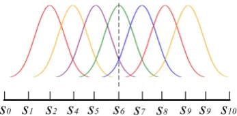
DOI: 10.4236/jcc.2018.612008 83 Journal of Computer and Communications whose value differs 0. As Figure 1 shows, at knot s6, only the three functions intersect with the dash line have values not equal 0, and a, b, care used to denote the values of these 3 functions. The local support property of B-Spline curve de-termines that only part of the curves on surface are referenced when regulating control vertices of one certain cross section curve, which is the source of local refinement.

So for cross section curve C tr( ), equation as (3.2) indicating the relationship of the curve and its equivalent position on the T-Spline surface can be deduced:



1, 1, , , 1, 1,

1, , 1,

( ) ( ) ( , )

( ) ( )+ ( )

( ) ( )+ ( )

r

rl r rl

rl r rl

j

r j r

j I

r j r j r j r j r j r j

j I j I j I

rl rr

r j j r j j r j j

j I j I j I

C t V N t P s t

X B t W B t Y B t

a X N t b W N t c Y N t

∈ − − + + ∈ ∈ ∈ − + ∈ ∈ ∈ = = = + = +

∑

∑

∑

∑

∑

∑

∑

In (3.2), Wr j, denotes the control vertices after regulation, Ir, Irr denote the control vertices’ subscript index set of left intermediate section curve, cross section curve and right intermediate section curve. In this method, one prere-quisite is Irl ⊆Ir, Irr ⊆Ir, which means the cross section curve C tr( ) has more knots than both the left and right intermediate section curves, for this guarantees that the basic functions of these two intermediate section curves can be expressed as the linear combination of C tr( )’s basis functions thus Equation (3.2) is solvable [5]. If the two intermediate section curves on the left and right have the same knot vector as the section curve, then the basic functions rl( )

j

N t , ( )

rr j

N t and N tj( ) are coincident, under which (3.3) can be simplified as a li-near equation in (3.3):

( )

j j j j r

V =aX +bW cY j I+ ∈ _(3.3)

For the situation that the intermediate section curves and the cross section curve have different knot vector, knot insertion in [6] can be used to express the

( )

rl j

N t and rr( )

j

N t as the linear combination of N tj( ). Then Equation (3.4) can be given.

' ' '_{( )}

j j j j r

V =aX +bW cY j I+ ∈ _(3.4) Here '

j

X and '

j

Y are the new control vertices of intermediate curves com-puted by knot insertion. By the solution of Equations (3.3) and (3.4), the sur-face’s new control vertices can be obtained which can define the T-Spline surface interpolating the given cross section curves.

DOI: 10.4236/jcc.2018.612008 84 Journal of Computer and Communications

Drawback of Local T-Spline Skinning

Obviously in the scheme given above that the intermediate section curves’ con-trol vertices play an important role in T-Spline surface modeling. A. Nasri [5] gave a method to generate the intermediate section curves by cross section curves. But this method has its defects: usually the number of control vertices of the intermediate section curves is not enough to embody the surface’s shape feature between section curves, resulting in wiggles on the final surface, which are difficult to eliminate just by regulating the surface’s control vertices. As the case shown in Figure 2, dramatic wiggles appear on the skinning surface and the shape of the final surface is far from that of the designer’s expectation [8].

4. Shape Preservation Local T-Spline Surface Skinning

4.1. Key Points of Shape Preservation

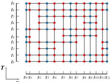
Focus on the existing problem in the above method, M. Oh et al. raised local T-Spline skinning method capable of shape preservation [8]. The key points of this method rely in that for each cross section curve, add one more intermediate section curve on both its left and right. The knot vector of the intermediate sec-tion curves is the same as that of the cross secsec-tion curve. In Figure 3 one exam-ple of the T-mesh capable of shape preservation is demonstrated. In this T-mesh, the blue knot vectors are those of cross section curves, and red ones are of in-termediate section curves.

(a) (b)

Figure 2. Surface wiggles and the ideal skinning surface. (a) Surface wiggles; (b) The ideal skinning surface.

DOI: 10.4236/jcc.2018.612008 85 Journal of Computer and Communications The introduction of two intermediate section curves makes it easier to control the T-Spline surface’s shape around the cross section curve. The positions of in-termediate section curves’ control vertices are still very important, and in this method they can be regulated locally to achieve the wanted smoothness of T-Spline skinning surface. Compared with A. Nasri’s work, this method is supe-rior in the follows: 1) The shape of the T-Spline surface around cross section curves are easier to control. More knots mean more degrees of freedom, and more flexibility for surface morphing. 2) The surface can keep the shape of cross section curves effectively. The information of intermediate section curves reflects the shape variation tendency of the surface between two cross section curves. 3) Easy implementation of the control vertices’ regulation algorithms. For interme-diate section curves exist on both the left and right of the cross section curve, and the knot vector of the intermediate section curve is the same as the cross section curve’s, only the linear equation as (3.3) is enough for the problem solv-ing.

4.2. The Generation of Intermediate Section Curves and the Shape

Keeping

How to generate the intermediate section curves is the most important mission in the local T-Spline surface skinning capable of shape preservation. M. Oh raised an intermediate section curve generation algorithm based on linear in-terpolation [8]. The main point of this algorithm can be illustrated in Figure 4. The first step is to calculate sample points on cross section curve in the direction of parameter t, i.e. calculate the coordinates of a series of points on cross section curve with given knots. The knots can be given evenly, and more sample points can be obtained with less knot interval. Then linearly interpolating these sample points in the direction of s parameter to calculate more points as the points on intermediate section curves. At last, fit these points to obtain the control vertices of the intermediate section curves.

On general occasions the above method can have satisfying results. But wig-gles can also occur on some occasions, for the control vertices of intermediate section curves calculated by reverse algorithm may not reflect the coordinates of the cross section curves’ control vertices properly, thus the surface will be stretched for some degree in these areas and leads to wiggles.

DOI: 10.4236/jcc.2018.612008 86 Journal of Computer and Communications As in Figure 4, considerate distances between Vr j, and Vr j', may appear and this will result in the situation in Figure 5, i.e. severe wiggles appear in surface’s locals. To alleviate this phenomenon, M. Oh raised an algorithm of iterative re-verse calculation [8], which will compute the distance between surface and in-termediate section curve and by regulating the control vertices’ coordinates to minimize the wiggles. This method can derive good results but when the wiggles are heavy the iteration and regulation will increase the computation work needed for surface skinning.

Aiming to further improve the above method, a new algorithm for shape pre-servation T-Spline skinning surface is proposed below, which simplifies the gen-eration of intermediate section curves, and at the same time minimizes the wig-gles. Usually no iteration and reverse computation work is needed and if on some occasions is in need, the workload is lighter compared with the existing method.

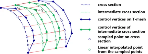
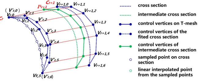
As in Figure 6, Cr and Cr+1 are two cross section curves, of which the control vertices are denoted as V ir i, ( =0,1,...,5) and Vr j, (j=0,1,...,6). In

or-der to insert the left intermediate section curve 1 1

r

I + (The green curve in the figure is intermediate section curve, wherein the superscript 1 denotes the left intermediate section curve and 2 denotes right one, the subscript r + 1 means that this intermediate section curve corresponds with the ( 1)r+ _{th cross section} curve), sample points on curve Cr are firstly computed, then these points are used to fit a curve, of which the number of control vertices are the same as that of the curve Cr+1, and obtaining control vertices Vr j', (j=0,1,...,6). The inter-mediate section curve’s control points can be computed by the linear interpola-tion of '

,

r j

V and Vr+1,j. At last, the knot vector of intermediate cure is required to be the same as that of Cr+1, then the left intermediate section curve Cr+1 is achieved.

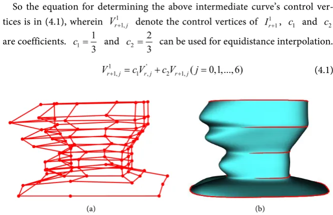
So the equation for determining the above intermediate curve’s control ver-tices is in (4.1), wherein 1

1,

r j

V+ denote the control vertices of I1r+1, c1 and c2 are coefficients. c1=1₃ and c2=2₃ can be used for equidistance interpolation.

1 '

1, 1 , 2 1, ( 0,1,...,6)

r j r j r j

V+ =c V +c V+ j= (4.1)

(a) (b)

DOI: 10.4236/jcc.2018.612008 87 Journal of Computer and Communications

Figure 6. Insertion of intermediate section curve

I

In the same way, Figure 7 demonstrates the process of inserting 2

r

I as Cr’s right intermediate curve. The first step is to compute the sample points on curve

1

r

C+ , then fitting these sample points, on condition that the number of fitting curve’s control vertices is the same as that of Cr, at last compute intermediate section curve 2

r

I ’s control vertices by linearly interpolation of fitting curve’s control vertices '

1,

r i

V+ and Cr’s control vertices Vr i, . The knot vector of

inter-mediate section curve is the same as curve Cr.

Repeat the above operation on all the cross section curves then all the curves needed for T-mesh generation are obtained. Using this method to compute the intermediate section curves can keep the shape trend of cross section curves’ control vertices, thus reducing the wiggles in M. Oh’s method and reflect the cross section curves’ shape in the final surface. It is noticed that M. Oh’s method on Figure 8 doesn’t perform the algorithm in reference [8].

5. Results & Discussion

Several examples are given below to show the effectiveness of the shape preser-vation local T-Spline skinning method proposed in this paper (Figure 9 and Figure 10).

In this paper, a new algorithm for shape preservation local T-Spline skinning is given. In this algorithm, new intermediate section curves are to be inserted between cross section curves. By sampling points on the cross section curves, and use them to reverse compute control vertices, the intermediate section curves’ control vertices can be obtained by linear interpolating these control vertices, and their knot vectors are the same with the corresponding section curves. An error decided by the fitting algorithm will be introduced in the process of con-trol vertices’ reverse computation. The advantage of this algorithm exists in that it sharply minimizes the possibility of the wiggles and its computation workload is light. And comparing with the method of A. Nasri [5], this method increases the number of control vertices.

DOI: 10.4236/jcc.2018.612008 88 Journal of Computer and Communications

Figure 7. Insert intermediate section curve

I

(a) (b)

Figure 8. Comparison of the two methods. (a) M. Oh’s method; (b) This paper’s method.

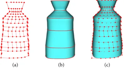
(a) (b) (c)

Figure 9. T-Spline skinning surface: example 2. (a) T-mesh in 3D space; (b) T-Spline skin-ning surface; (c) T-mesh and T-Spline surface.

(a) (b) (c)

DOI: 10.4236/jcc.2018.612008 89 Journal of Computer and Communications this paper can result in a T-Spline skinning surface of which the number of con-trol vertices is O kn(3 ) [2]. Usually the number of cross section curves are over 3, so even the algorithm here increases the number of control vertices than A. Nasri’s method, it’s still less than in the traditional NURBS skinning. And the newly increased control vertices firmly decrease the surface wiggles as well as provide more flexibility in the surface representation. Also the computation workload is decreased in this method, and no knot insertion is needed for the surface smoothing.

In future work, more cases will be tested, and if for some occasions the smoothness cannot be satisfying, maybe special work for surface smoothing will be combined with this method to improve its adaptability.

Acknowledgements

The authors would like to acknowledge the support by the Natural Science Foundation of China (Project No.61572056).

Conflicts of Interest

The authors declare no conflicts of interest regarding the publication of this pa-per.

References

[1] Piegl, L. and Tiller, W. (2010) The NURBS Book. Tsinghua University Press, Bei-jing.

[2] Piegl, L.A. and Tiller, W. (2002) Surface Skinning Revisited. Visual Computer, 18, 273-283. https://link.springer.com/article/10.1007/s003710100156

https://doi.org/10.1007/s003710100156

[3] Sederberg, T.W., Zheng, J., Bakenov, A., et al. (2003) T-Splines and T-NURCCs. ACM Transactions on Graphics, 22, 477-484.

https://www.researchgate.net/publication/234827617_T-splines_and_T-NURCCs

https://doi.org/10.1145/882262.882295

[4] Sederberg, T.W., Cardon, D.L., Finnigan, G.T., et al. (2004) T-Spline Simplification and Local Refinement. ACM Transactions on Graphics, 23, 276-283.

https://www.researchgate.net/publication/234780696_T-spline_simplification_and_

local_refinement

https://doi.org/10.1145/1015706.1015715

[5] Nasri, A. (2012) Local T-Spline Surface Skinning. Visual Computer, 28, 787-797.

https://link.springer.com/article/10.1007/s00371-012-0692-1

https://doi.org/10.1007/s00371-012-0692-1

[6] Yang, X. and Zheng, J. (2012) Approximate T-Spline Surface Skinning. Comput-er-Aided Design, 44, 1269-1276. https://doi.org/10.1016/j.cad.2012.07.003

https://www.researchgate.net/publication/256688182_Approximate_T-spline_surfa

ce_skinning?ev=prf_high

[7] Li, Y., Chen, W., Cai, Y., et al. (2015) Surface Skinning Using Periodic T-Spline in Semi-NURBS Form. Journal of Computational and Applied Mathematics, 273, 116-131. https://doi.org/10.1016/j.cam.2014.05.026

DOI: 10.4236/jcc.2018.612008 90 Journal of Computer and Communications

odic_T-spline_in_semi-NURBS_form

[8] Oh, M.J., Roh, M.I. and Kim, T.W. (2018) Local T-Spline Surface Skinning with Shape Preservation. Computer-Aided Design.

https://www.researchgate.net/publication/325065815_Local_T-spline_surface_skinn