Deployment Optimization Strategy for a Two Tier Wireless Visual Sensor Network

(1)

Deployment Optimization Strategy for a Two-Tier

Wireless Visual Sensor Network

Hailong Li, Vaibhav Pandit, Dharma P. Agrawal

School of Computing Sciences and Informatics University of Cincinnati, Cincinnati, USA Email: {lih6, panditvv}@mail.uc.edu, dpa@cs.uc.edu

Received January 9, 2012; revised February 22, 2012; accepted March 14,2012

ABSTRACT

Wireless visual sensor network (VSN) can be said to be a special class of wireless sensor network (WSN) with smart- cameras. Due to its visual sensing capability, it has become an effective tool for applications such as large area surveillance, environmental monitoring and objects tracking. Different from a conventional WSN, VSN typically includes relatively expensive camera sensors, enhanced flash memory and a powerful CPU. While energy consumption is dominated primarily by data transmission and reception, VSN consumes extra power onimage sensing, processing and stor-ing operations. The well-known energy-hole problem of WSNs has a drastic impact on the lifetime of VSN, because of the additional energy consumption of a VSN. Most prior research on VSN energy issues are primarily focused on a sin-gle device or a given specific scenario. In this paper, we propose a novel optimal two-tier deployment strategy for a large scale VSN. Our two-tier VSN architecture includes tier-1 sensing network with visual sensor nodes (VNs) and tier-2 network having only relay nodes (RNs). While sensing network mainly performs image data collection, relay network only for wards image data packets to the central sink node. We use uniform random distribution of VNs to minimize the cost of VSN and RNs are deployed following two dimensional Gaussian distribution so as to avoid en-ergy-hole problem. Algorithms are also introduced that optimizes deployment parameters and are shown to enhance the lifetime of the VSN in a cost effective manner.

Keywords: Energy-Hole Problem; Gaussian Distribution; Relay Node; 2-Tier Network; Visual Sensor Node; Wireless

Visual Sensor Network

1. Introduction

Wireless visual sensor network (VSN) can be considered to be one special type of wireless sensor network (WSN) with visual sensing capability. With development of cheap sensing devices, wireless networking and embedded com- puter, VSN has become a new technology with tremen- dous potential for many applications [1]. A VSN typically consists of smart cameras [2], processing chips and wireless transceivers. Besides image capturing function, each smart camera is capable of extracting information from images. Processing chips could do further image processing operations such as image compression or mak- ing decisions based on the image data. Wireless trans- ceiver takes care of forwarding image task to the network sink node or the base station (BS). To achieve such a powerful image data handling capability, each visual sensor (VN) is typically equipped with relatively expensive cameras, additional flash memory and more powerful CPU as compared to a conventional wireless sensor. Nu- merous applications for VSNs have been conceived such as surveillance of public places or remote areas, envi-

ronments monitoring for animal habitats or hazardous areas, smarthomes for babies and elderly people, and vir- tual reality [3].

Although a lot of issues in VSN have been studied, there are still many challenges for a VSN [4]. Since VNs are battery-operated device, energy management is one of the important research topics in the VSN community. Among most prior research on VSN, the energy management issue is primarily focused on a single device or a given specific scenario. The notorious energy hole problem [5,6] inherited from WSN research for large scale uniform random distribution VSN has been totally ignored in earlier work. Since wireless sensors need to relay data packets from each other, sensors close to the BS always consume more energy than the sensors located far away. Once close by sensor nodes run out power, the BS gets disconnected from the whole WSN.

(2)

operations. Because of such additional energy consumption, the energy-hole problem of WSNs has a drastic in- fluence on the lifetime of a VSN. In [7], Wang et al. have analyzed the coverage and life time of Gaussian distributed WSN and proposes an optimized deployment strategy that maximizes the lifetime of a WSN. However, since VNs are relatively more expensive than other conventional sensors (e.g., temperature and humidity sensors), deploying more redundant VNs in the inner area following a Gaussian distribution only for energy backup, does not seem to be a cost efficient option. Therefore, Gaussian distribution could not be utilized while deploying VNs.

In this paper, we propose a two-tier deployment strategy for wireless VSN. For a large scale deployment as a uniform random distribution is a cost efficient scheme, especially when there is no previous knowledge about the physical parameters, even though the performance is limited by the energy-hole problem. Therefore, we deploy VNs as a sensing network following a uniform random distribution in a given area, which sense visual data. Since VNs could form a complete WSN, we would like to call it as tier-1 network. In addition to VNs, we propose to deploy another type of sensor nodes called relay nodes (RNs) concentrically distributed parallel to the sensing network. These RNs provides the function of relaying image data to the BS or the sink node.

To take care of the energy hold problem, the relay network deployment basically follows a two-dimensional Gaussian distribution, with mean (μx, μy) at the center of sensing network Although RNs do not generate data, they create acommunication relay infrastructure and we call it as a tier-2 network. Then, the sensing network and the relay network constitute a two-tier wireless VSN, with BS at the center of the monitored region, as illus- trated in Figure 1.

[image:2.595.310.538.84.262.2]

Note that as the monitoring tasks and the regions vary, the VSN deployment needs to be designed accordingly. Among many factors, monitored region should be the most important factor to be analyzed. For tier-1 sensing network, an approximated shape of the monitored area is not important since VNs should be distributed in the same symmetrical manner no matter what the shape is. On the contrary, the parameters of the tier-2 relay network standard deviation σ depends on the shape of the region. If the shape of monitored region can be approximated by a circle, square or equilateral triangle, Gaussian distributed relay topology with σx= σycould fit the area very well. If the shape of monitored region is similar to a rectangle or an ellipse, Gaussian distribution with σx≠σy could be an appropriate choice for such a scenario. For simplicity, we call two-tier VSN with σx = σy Gaussian distributed relay network as a Circular VSN, and use Elliptical VSN to represent two-tier VSN with σx ≠ σy

Figure 1. Two-tier wireless visual sensor network constructed from Base Station (BS), Visual Sensor Node (VN) and Relay Node (RN).

Gaussian distributed relay network in this paper. Undoubtedly, for the tier-1 sensing network, the VNs deployment strategy is usually based on the monitoring objective. The monitored area, and the VNs sensing range are preplanned according to special features of the VSN project and the only question needed to be an- swered is:

 How many VNs should be deployed for the monitored region to satisfy the coverage requirement? For tier-2 relay network, there are two key questions that need to be addressed before deployment:

 How many RNs should be deployed within the tier-1 sensing network?

 How to configure the parameters of the Gaussian distributed RNs so as to optimize the performance? To answer these questions, theoretical analysis and modeling for two-tier VSN is needed. We choose lifetime and cost as our objectives to measure the performance of VSN under different deployment strategies. Analy- sis on coverage and connectivity of two-tier VSN is nec-essary right at the beginning. Thereafter, the optimization problem can be defined in terms of lifetime and cost of the VSN so as to reflect the optimized deployment pa-rameters. The main contributions of our work here are as follows:

 We present an analytical model for the coverage and the connectivity of a Circular VSN and establish a relationship between the network requirements and VSN deployment parameters from the geometry point of view.

 We provide a new formalism to model an Elliptical VSN and derive an analytical model.

(3)

ters.

 Based on the shape of the monitored region, we suggest a large scale VSN should be divided into several small VSNs for monitoring different types of tasks. The rest of the paper is organized as follows. Related works are discussed in Section 2. The system model is introduced in Section 3. In Section 4, we analyze the coverage and connectivity of Circular VSN. The coverage and connectivity of Elliptical VSN are discussed in Section 5. Then, in Section 6, we propose deployment strategies for a large scale VSN with optimization in mind. Finally, Section 6 concludes the paper.

2. Related Works

WSN related topics have been extensively studied in recent years, and many researchers have provided sub- stantial theoretical and practical results. Some theories and algorithms for WSN could be directly applied to VSN. However, many challenging issues are still open for VSN. In this section, we would like to review energy management schemes for VSN and lifetime optimization strategies for WSN.

2.1. Energy Management of Wireless Visual Sensor Network

Charfi et al. [4] discussed several research issues on the optimization of smart camera coverage, low-power image processing, VSN architecture, and wireless communication. Since a wireless sensor in a VSN is a battery- driven device, energy management is always an important research topic. Due to severe energy constraints on VSN, many works have been done on how to use the energy efficiently. Coordinated Distributed Power Man- agement (CDPM) policy for VSN has been proposed by Zamora and Marculescu in [8]. Their CDPM policies include dynamic and adaptive timeout thresholds, hybrid CDPM, two-hop broadcast information dissemination, and remote wakeup.

Soro and Heinzelman [9] presented two camera selec- tion schemes in providing longer lifetime in a network. One scheme selects cameras that minimize the difference between captured images and the other scheme is based on choosing a VN by considering the energy constraints and the three-dimensional coverage. Since the data trans- mitted in a VSN are images captured by smart cameras and the amount of data has a huge impact on the energy consumed by data forwarding operation, image compression technique is one of the solutions for efficient energy management of a VSN.

Dagher in [10] analyzed the inter- and intra-sensor correlation for power-constrained VSN and proposed an algorithm using a compression scheme. Margi et al. [11] conducted an energy consumption experiment on a visual

sensor testbed to determine the power utilization for different image handling tasks. The results of their experiments provide a comprehensive understanding of energy consumption in a VSN.

Hadi et al. [12] proposed a two-tier topology for camera-based wireless multimedia sensor networks. A number of Non-camera sensor nodes with powerful CPU processing ability are deployed above the lower-tier visual sensor network to form a higher-tier network. To combine multiple images from lower-tier visual sensor nodes, higher-tier sensor nodes perform Image stitching to create a high-resolution image. Energy consumption is minimized by reducing the redundant data being for- warded for the overlapping areas covering multiple images.

To summarize, most prior VSN energy management research focused only on a single visual sensor node or a given specific scenario. To our knowledge, energy-hole issue has not been considered for a large scale VSN. Thus, our study focuses on solving energy-hole problem while increasing the lifetime of VSN with minimal cost.

2.2. Lifetime Optimization of Wireless Sensor Network

Many theoretical results about coverage, connectivity and lifetime have been proposed for randomly distributed large scale WSN. Uniform randomly distributed WSN has attracted more attention from researchers, since from a practical point of view; it is a good option for different sensing tasks, especially when there is no previous knowledge about the deployed area. But, the drawback of uni-form random distribution WSN is a well-known energy- hole problem for periodic data collection applications. Li

et al. [13] show that lifetime of a uniformly distributed WSN is limited by the sensor nodes one-hop away from the BS and they also suggest several schemes to mini-mize the impact of energy-hole problem.

In order to increase the data capacity of WSN, a non- uniform distribution strategy has been proposed by Lian

et al. in [14]. The results show that up to 90% of initial network energy is wasted when WSN becomes disconnected, when the sensor nodes close to the BS runs out of energy. Some controllable random distribution schemes are proposed to address the energy-hole problem. A strategy is provided by Wu et al. [15] to balance the energy depletion of a WSN. They propose to deploy sensors from outer area to inner area according to certain geometric proportion. Liu et al. [16] proposed a non- uniform deployment scheme for enhancing the lifetime of WSN. The results in [16] shows that the scheme can mostly take care of the energy-hole problem.

(4)

accurately controlled, which is impractical for some real applications. Zou et al. [17] proposed an idea that sensors could be distributed following two-dimensional Gaussian distribution without detailed analysis. Afterwards, Wang

et al. [7] provided a comprehensive analysis on the coverage and the lifetime of a two-dimensional Gaussian distributed WSN and optimization algorithms are provided to find the optimal deployment parameters that increase the lifetime of WSN so as to relax the impact of the energy-hole problem.

Although all existing schemes provided desirable results for WSNs, we feel that they cannot be directly applied to VSN deployment. The essences of these schemes are based on adding more sensors closer to the BS to handle data forwarding tasks. These ideas fit well in a WSN environment, especially when the sensor hardware cost keeps going down, benefiting from the advances in the sensor industry. But, VNs in VSN are relatively expensive sensors with smart cameras. Simply deploying more VNs for energy backup will definitely increase the cost and is not an acceptable option for an optimal design of a monitoring task. Therefore, we propose two-tier VSN strategy to simultaneously relax the energy-hole and cost wastage problems.

In the following section we will describe the network sensor system model by first describing the Network deployment model, the energy model and then the sensing and connectivity model.

3. Sensor System Models

In this section, we introduce models for the network deployment, sensor energy, sensing and connectivity for wireless VSNs.

3.1. Network Deployment Models

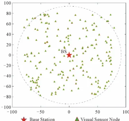
1) Random Distribution Sensing Network: Consider that a large number of M VNs need to be deployed in a two- dimensional geographical region D, and the BS is located at the center, forming our tier-1 sensing network. We assume that the VNs are deployed uniformly and independently, and we could call it as uniform VSN for short.

When prior knowledge of the region is not available, such a random deployment could be an effective method. Under this scenario, location of VNs could be modeled as a stationary 2-D Poisson point process [18]. Denote the number of visual sensors in field D as N (D), which follows the Poisson distribution as:

 







_!e



k D

D P N D k

k



 

  (1)

where λ is density of the Poisson point process and D

is the area of region D. An example of a two-dimensional

randomly distributed sensor network is shown in Figure 2 with BS at the center.

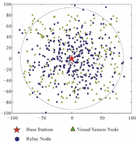
2) Gaussian Distribution Relay Network: We consider that a network with N relay nodes are deployed in a two- dimensional plane, which is called tier-2 or relay network in this paper. The RNs deployment pattern follows two- dimensional Gaussian distribution as:

 

  2 2

2 2

1

, e

2π

i i x y

x x y y

x y

f x y  

 

   

 , (2)

where (xi, yi) is the position of the BS and σxandσy are the standard deviation for x and y directions. To simplify the analysis, let the sink node position be xi = 0, yi = 0, then we have:

 

2 2

1

, e

2π

x y

f x y  

 

 

 

_  

 .₍₃₎

A two-dimensional Gaussian distribution with σx = σy relay network example is shown in Figure 3 with BS at

the center.

3.2. Energy Models

[image:4.595.310.535.484.696.2]

1) Relay Node Energy Models:Since RNs do not generate any data, energy consumption is dominated only by the radio communication system (i.e., data transmission and reception tasks). When RNs relay image data, we can determine the energy consumption using the first order radio model described in [19]. The energy Et(m, d) consumed by transmitting m-bit packet to distance d can be given by:

(5)

[image:5.595.58.286.83.289.2]

Figure 3. Two-dimensional gaussian randomly distributed relay network with Base Station (BS) and Relay Node (RN).



_,



2

t elec amp

E m d E  m   m d (4) where Eelec is the energy cost to activate the transmitter or receiver circuit and amp is for the communication transmitter amplifier. During reception by a RN, energy consumption only depends on the data load. So, total energy consumed Er (m) can be given by:



 

,

r elec

E m E m (5) where Eelec is the same as Equation (4). Suppose VNs collect L' bits of image data in each sampling cycle, and the image data must be divided into several small m bits data packets to be communicated from VNs to the BS. With additional header overhead bits, let us use notation

L, where L > L', for total bits of packets in every data collection cycle generated by each VN. When the transmission distance d is set as the sensor radio transmission range rc, the total transmission energy used for each sampling cycle can be computed by:

 

,

t t

E L K L (6)

where 2

t elec amp c

K E  r , and we can calculate the reception energy Er (L) as

 

,

r r

E L K L (7) where Kr Eelec. Although RNs and VNs have different functions, their radio system certainly can be the same hardware as RNs. Thus, Equations (6) and (7) can also be used for VNs communication energy calculation.

2) Visual Sensor Energy Models: Typically, WSN include relatively simple sensors, such as temperature, humidity and light sensors, etc., and energy consumption is dominated by the wireless transmission and reception of WSN radio communication system. However, due to the

significant difference in sensing hardware (i.e., cameras) of VSN, the common energy consumption model in WSN apparently cannot be utilized for VSN energy calculation. The energy measurement experiment for VN in [11] provides us a comprehensive understanding of energy consumption during visual sensor running session. Margi et al. [11] conducted measurements on their Meer- kats testbed (Crossbow’s Stargates, Orinoco Gold 802.11b PCMCIA wireless card and Logitech QuickCam Pro4000 webcam). The main energy consumption tasks of VN in one sampling operation cycle includes:

 Sensing Energy Ee: Energy consumed for collecting image data by a camera

 Storage Energy Es: Energy used for writing and read- ing image data on a flash memory.

 Processing Energy Ep: Energy consumed in perform- ing Fourier Transform for images.

 Transmission Energy Et: Energy in sending image data to the neighboring nodes.

 Reception Energy Er: Energy consumed for reception of neighboring wireless nodes.

The transmission energy Et(L) and reception energy

Et(L) are already considered in the RNs energy model. So, we focus on other aspects of the energy model. The sensing, storage and processing energy models would vary for different sensor hardware and an accurate energy consumption model is beyond the scope of this paper. But, based on the observation of the experiments data [11] and the nature of circuit, we use the first order energy model to estimate the energy consumption for sensing, storage and processing tasks as:

 

,

e e

E L K L (8)

 

,

s s

E L K L (9)

 

.

p p

E L K L (10)

3.3. Sensing and Connectivity Models

1) Network Sensing Range Model: For research in WSN, a circular shaped coverage by a sensor is always assumed. On the contrary, smart cameras on VNs normally cover less than 180˚ area. However, since smart cameras shooting angle can be remotely adjusted to a proper direction by the network operator, we still use a circular shape to estimate the coverage of our proposed two-tier network. VNs are randomly and independently deployed in a two-dimensional region. Liu et al. [18] show that for such a randomly deployed sensor network in a two-dimensional infinite plane, the probability fa that a point is covered by at least one sensor is as follows:

2

π 1 e rs, a

(6)

each sensor node. Sensing task is performed only by VNs. Thus, Equation (11) can be utilized for our random distribution tier-1 sensing network directly and minimal number of VNs for a given region can be estimated.

2) Network Transmission Range Model:In a random uniform distribution network, Bettstetter in [20] showed a relationship between the sensor transmission range rc and the network connectivity as:



1/



ln 1 ,

π

n c

p r



 

 (12)

where p is the possibility that none of the sensor node in the network is isolated, n is the total number of sensor nodes deployed in the large area A satisfying 2_π

c

Ar , and  n A is the node density. Equation (12) is only for random uniform distribution, while, this can be still useful in our Gaussian distribution relay network analysis of Section 4.

4. Coverage and Connectivity of Circular

Wireless Visual Sensor Network

In this section, we present an analysis for Circular VSN to satisfy the basic network requirement of both the coverage and the connectivity. We consider a two-tier wireless visual sensor network: tier-1 sensing network with random uniform distribution consists of VN with a sensing range rs and transmission range of rc; tier-2 relay network with random Gaussian distribution consists of RNs with the same transmission range rc. In this section, we analyze Circular VSN by modifying Equation (3) as:

 

2 2

2

2 2

1

, e

2π

x y

f x y 



     _

 .₍₁₃₎

Two networks are concentric and have the same BS at the center point. Figure 4 shows an example of our de-

ployment strategy in a two-dimension plane with sink node (star) at the center, VNs as green triangles and RNs as blue dots. Next, we discuss a scheme of deploying the VNs and RNs to guarantee the coverage of the area and their connectivity to the BS.

4.1. Coverage of Circular VSN

Apparently, sensing function of a two-tier network is done only by the sensing network at tier-1. Coverage of two-tier network depends on uniformly distributed sensing network and coverage probability Ps can be given based on Equation (11) as:

2

π 1 e M rs A, s

[image:6.595.312.537.83.317.2]

P    (14) where M is the number of VNs and A is the area of monitored region. rs depends on the sensing capability of

Figure 4. An example of Circular VSN in monitored region with Base Station (BS), Visual Sensor Node (VN) and Relay Node (RN).

camera on VNs. Once rs is set based on visual task, coverage probability would increase when more VNs are deployed in a given area.

Assume the coverage requirement as *

s

P (e.g., 95%). To guarantee the coverage of tier-1 network, we need at least M VNs satisfying:

2

π *

1 e M rs A .

s s

P    P (15) Equation (15) provides a theory to support optimized cost for wireless VSN, while meeting the coverage requirement at the same time.

4.2. Connectivity of Circular VSN

VNs and RNs have the same radio hardware and transmission range rc and two sensors can communicate with each other if they are within each other’s distance rc which is a preplanned parameter. If rc is set too small, either the network connectivity is compromised or additional sensors ought to be deployed, adding to the cost. But, due to hardware limitations, rc cannot be adjusted arbitrarily and there is a maximal radio transmission range m limiting

c

r m

c c

r r . rc should be set to be a proper max value as long as wireless link quality could meet the requirements.

To analyze a Circular VSN, two-tier network is modeled as a disk as is done in [7]. The disk with radius R is divided to multiple annuli as shown in Figure 5, and the

(7)

[image:7.595.85.258.84.251.2]

Figure 5. Disk annuli division of a Circular VSN. from 1 to k where k R rc

r

. Then, any sensor node with distance d to the BS always falls inside ith annuli of disk if d satisfies





c. To consider

tier-1 network only, sensing network is divided into [1, 2, ···, k] annuli and since tier-1 network follows a uniform random distribution, VNs node density

1 c

i    r d i

s

 is the same in each annulus. Relay network is planned to be deployed concentrically to the sensing network and since the relay network follows a Gaussian distribution, inner annuli RNs node density r is larger than outer annuli node density.

We assume VNs only sense visual data and send packets to neighbouring RNs and VNs do not relay any packets. Rest of the packets forwarding need to be handled only by the relay network. Furthermore, all traffic from outer annulus i + 1 is distributed uniformly among the RNs in annulus i. This assumption requires an ideal routing mechanism in such a way that the traffic load from VNs is uniformly allocated to RNs in the same annulus and relaying traffic load is also allocated uniformly to RNs in one-hop annulus, which would balance the residual energy for all the RNs. Although Equation (12) is proposed for a uniform random distribution, we apply this model to calculate the network connectivity in each annulus after an appropriate annuli division of the whole region. Since annulus width _c , distribution of RNs inside each annulus is approximated as a uniform distribution.

r R

To guarantee the connectivity inside each annulus, we utilize Equation (12) with the scenario that each VN only send packets to RNs located in the same annulus. Then, if VNs send packets to one-hop annulus RNs, fewer RNs in the same annulus is needed and the network connectivity is still guaranteed. Network connectivity is a cru- cial requirement and worth more discussion. For each VN, connectivity of a two-tier network actually means connectivity of a large number of uniform random distributed RNs. Rewriting Equation (12) for annulus i as:



_π2



1 e irrc Ni,

i c

P _{ }  ₍₁₆₎ where Ni is the number of RNs in the annulus i and

r

i i i is i annulus node density of RNs. When

deployed target region and RNs radio transmission range

rc are given, Equation (16) indicates the relation between the connectivity probability and the number of deployed sensors.

N A

 

If the network connectivity requirement is satisfied in the outermost annulus k with Nk relay nodes, then the relay network can guarantee connectivity of the network, as all inner annuli of Gaussian distributed relay network have a higher node density than the outermost annulus. Assuming the network connectivity requirement is and outermost annulus k connectivity is , then we need at least relay nodes in annulus k satisfying:

*

c

P

k c

P

*

k

N





*

2

π *

1 e kr c k .

N r k

c c

P    P (17) With disk annuli modeling, we have a relation between

Nk and the total number N as:

 

, 1,

i i

N  N P  i k , (18) where Pi is the probability that a RN is in the ith annulus of VSN network and can be calculated by:

 

1, 1,

i i i

P FF  i k , (19)

where Fi indicates cumulative distribution function (CDF) of two-dimension Gaussian distribution over a circular area, whose radius is irc. If we plot the 2D Gaussian distribution f(x, y) as Z axis direction in a three-dimension space X, Y, Z, itis clear that Fi is the volume enclosed by

XY plane and Gaussian distribution function f(x, y). As in

Figure 6, the mesh represent probability distribution of

RNs among X, Y plane, and the volume of purple solid “ring” object is the cumulative probability of RNs with annulus i. Thus, Pi can be calculated by the volume of the “purple ring” enclosed by annulus i area on XY plane and Gaussian function f(x, y). f(x, y) is probability distribution function, so it is always positive. And since f(x, y) =

f(–x, y) = f(x, –y) = f(–x, –y), f(x, y) is symmetric to X, Y

axis. The whole volume enclosed by f(x, y) boundary is four times of the volume in the first octant (X+_,_Y+_,_Z+_). Then, we can compute Fi based on the rules in calculus application in geometry as:





 

2 2

2 2 ₂

, , ₂

2

0 0

1

4 4 e

2π

c c

x y ir ir x

X Y Z

i i d d .

F F  x



   _   _  

 

_{ }

y (2

With the help of polar coordinates transformation, ha

0)

we ve:

2 2 _{2 2}

2 ₂

π

2 ₂

2 2

0 0

2

e d d 1 e

π

c _c

c

i r _{i r}

ir i

F  R R _ 



_ _

  

(8)

[image:8.595.60.287.84.256.2]

Figure 6. Ring interpretation of Piin a 3D space.

From Equations (19) and (21), we have:

 

 

2 2 2 2

1 c c

i r i r

2 2

1, .k

 

(22)

Based on Equations (17)-(22), we establish a relation between total number of RNs and the connect

quirement as:

2 2

1 e e ,

i i i

P F F   i



     

ivity re-



_π2



_*

1 e k c k k

NP NP r A k

c c

P    P (23)

where





2 2 2 2

2 2

1

exp exp

2

c c

k

k r k r

P



 _  _ _

 

   

2

  _ _

 

the area of annulus k.

5. Coverage and Connectivity of Elliptical

ensor Network

El-

ig- ur

Elliptical VSN k. Thus, Equation overage probability

 and Ak is

Wireless Visual S

In this section, the coverage and the connectivity of liptical VSN is discussed. One example is shown in F

e 7 as an ellipse-shape two-tier VSN.

5.1. Coverage of Elliptical VSN

Similar Circular VSN, coverage of two-tier only depends on tier-1 sensing networ (14) can be used for computing the c

of Elliptical VSN. Also, if we have the coverage prob-ability requirement *

s

P , we can utilize Equation (15) to calculate required minimal number of VNs in the sensing network.

5.2. Connectivity of Elliptical VSN

Different from a Circular VSN, tier-2 relay network de- wo-dimensional (3) with a mean ployment of Elliptical VSN follows t

Gaussian distribution following Equation

of (xi, yi) at the center of monitored region and standard variations (σx ≠ σy). To analyze an Elliptical VSN, it

could be modeled as an ellipse shape:

2 2

2 2 1,

x y

a b  (24)

where a and b are half of the ellipse’s major and minor axes respectively. Then, similar to

malism in Section 4, we can divide the whole area into the disk annuli for-

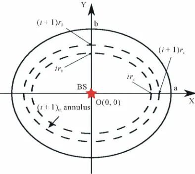
multiple annuli as shown in Figure 8. The center of el-

[image:8.595.308.538.266.492.2]

lipse is at the origin of XY plane, where the BS is located. To guarantee the connectivity of VSN, we designed ellipse division as follows. Without losing generality, we assume a > b for the whole VSN. We divide a on the positive X axis first into multiple line segments with width of rc, then we have k a rc line segment on

Figure 7. An example of Elliptical VSN in monitored region with Base Station (BS), Visual Sensor Node (VN) and Relay Node (RN).

[image:8.595.324.521.541.717.2]

(9)

positive X axis. Second, minor axes of VSN on positive Y

axis is cut into k line segment with width rbb k. Fi- nally, irc and irb, where i

 

1,k

f ellipse t a multip

, are used as half of the major and minor axes o o build ellipses in XY

plane. Now, we have le elliptical annuli VSN. Since b rc, any no

e-hop ann on, tier-1

r b ka k de in annulus i could transmit packets to on ulus towards the BS. Similar to the disk divisi network is divided into



1, 2, , k



annuli and VNs node density s n

is the same nulus. Tier-2 inner a nuli RNs node in each an

density r

network’s



ea

is larger th ter annu e density,

ch annulu de de

an the ou s, RNs no

li nod nsity

but within r is the

s

the ity requ t is

and we need at least Nk relay nodes in the annulus k

isfyi od-

same as l Assumin

ong a

g c

r a

networ .

k connectiv iremen *

c

P

at- s ng Equation (17). Similar to the disk division m eling, Fi can be calculated by integrating as:



2 2 2 2 2



2 1 ₂22 ₂22

0 0

4 e d d .

2π

c c b b c x y

x y ir i r r r x r

i

x y

F   x y

 

 

 

_  _

 _ _



_{ }

(25)

With dinates:

 

ellipse polar coor

 



 

2



2 ,

cos sin c b b c ir ir r ir ir     

 (26)

we can transform Equation (2) to:

      2 2 2 2 cos sin 2 e R R F    π

2 x 2 y

r  

2

0 0 d d .

π

i

x y

R R 

 

 

(

Finally, we can obtain Fi using:

   27)

 

2 2 2 π 2 0 2 cos sin 1 d ,

π ( )

b c

i

x y

r r

F  

2 2 2

1 exp i r rc b 

             



w     (28)

here

 

2 2

cos sin

Γ

2 x 2 y

 



  uation (28) can be

solved with a numerical integral method by

adaptive recursive Simpson’s rule. Based on Equations

  . Eq

following an

(19) and (28), we have:

 

1, 1,

i i i

P F F  i k . (29)

With Equations (28) and (29), we obtain a rela tween the number of RNs N and connectivity requi men

tion be- re- ts P_c* as:



_π2



_*

1 e NP rk c Ak NPk .

k

c c

P _{ }  _P ₍₃₀₎

6. Deployment Optimization of Large Sc

Wireless Visual Sensor Network

In Section 4 and Section 5, we analyzed the coverage and

rement of at least distributed tier-1 sensin

small value, then we need additional RNs to satisfy the connectivity r

wo

en , and the cost of RNs and VNs in the outer area simply become useless. Therefo

tion, we proposed optimal deployment str

of the lifetime and the cost for both Circular VSN and - tiv

ale

connectivity requi M VNs in a uni-

formly g network and Nk RNs in

annulus k of Gaussian distributed tier-2 relay network. For tier-2 relay network, choosing N and σ of Gaussian distribution in a cost efficient manner is challenging. If we choose σas a relative

equirement, which uld add to the cost. On the other hand, for certain number N RNs, if we choose a too large σ, the lifetime of network is reduced because of the energy-hole problem in the c ter area

re, in this sec- ategies in term

Elliptical VSN satisfying the coverage and the connec ity constraints.

6.1. Optimal Deployment Strategy for Circular VSN

Suppose we have M VNs and N RNs in a two-tier network deployed in the monitored region and divided into multiple annuluses. Each wireless node has the same initial energy level E0. The traffic pattern we considered implies that each visual sensor periodically senses image data and send to sink node located at the center of the network. Data collection interval of sensing network is denoted by 

 

t . In each data collection cycle, each VN generates L bits image data and RNs have the responsi-bility to forward them image to the sink node. We neglect the energy consumed by other network in the communication procedure, such as routing, MAC collisions, and assisting information exchange.

We use the notation _Ts_{to indicate the lifetime of}_i_th

annulus VNs and since all VNs follow the same data g and itting) in each cycle, VNs will deplete their collection procedure (i.e., sensing, storing, processin

transm

energy at the same time. Based on the energy model of section 3, VNs lifetime can be estimated by:

 

0

 

   

.

s

s e p t

E

T t

E L E L E L E L 



   (31)

For analyzing tier-2 relay network, an energy balanced ideal routing scheme is assumed, which allocates traffic load equally Ns. Thus, energy consumption rate for all RNs in each annulus are the same. Since RNs do not generate any data, the traffic load RNs received is equal to traffic load they transmit. We assume all the traffic load in annulus i from VNs are allocated on the same annulus RNs. So, a larger number of

to R

(10)

1 2,3, , k s j j 2 1, i _k s j j

A L i k

   _ _ _  



 Load

A L i      _ _ _ 



(32)

where Ai is area of annulus i and can be computed easily with _π 2



_{2 1}



c

r i , and _s_{is the node density of VNs}

and can be calculated by _s __{M A}_{. Since one-hop}

away VNs can directly send image data to BS, workload of RNs in annulus 1 and 2 are the same, i.e., Load1 =

Load2. Then, the total energy consumed in one data collection cycle can be expressed as:

.

i t i r i

E K Load K Load (33) We have Ni out of N RNs deployed in annulus i expressed as in Equation (18). Let r

i

T be the lifetime of RNs in i annulus and can be estimated as in [7] with Equations (32) and (33):

 

0 0 _.

r i i

i

i i

E N E N P

T t

E  E 

  

  t (34)

Lifetime T of two-tier network is defined as the time period when the battery-driven sensing network and the

. In other f

e of the n

relay network are running simultaneously in all [1, k] annuli words, i any annulus VNs or RNs runs out of initial power E0, lifetim etwork ends. If Ti denotes lifetime of annulus i network, our VSN lifetime

T is calculated by:





 

min min s, r , 1, .

i i

T  T  T T  i k (35) We use the notation Cr and Cs for the cos

an

age and connectivity requirements

t of each RN d VN, respectively. Then, the total cost of sensor devices denoted by C can be computed as:

.

s r

C C M C N  (36) With the knowledge of cover

*

s P

odele

and , our deployment o can be m d by following objective strain * c P the ptimization and con- ts:





 

* *

: min , , 1,

: (7) : . (8) s r i s r s s k c c

Maximize T T T i k

Minimize C C M C N

P P Subjectto P P          _  (37)

Coverage and connectivity constraints are shown by Equations (15) and (17). The multi-objective

tion problem modeled in Equation (37) typical tra

optimiza-ly can be nslated into a single objective optimization after nor-malization as:

: ln ln

* s s * : . (11) k c c (10)

Maximize W T C

P P Subjectto P P         _ 

where α, β are the wei ts of the corresponding two objectives, representing which objective is more important for deploym

gh

ent of VSN. Logarithm function is used to normalize two objectives and reduce the impact of individual attribute scale. For example, if the cost C is a larg number and T is a small one, then without lo

function, our objective will be dominated by the cost only. With logarithm function, we have

(38)

e garithm









1 2 1 2 1 2

1 1

2 2

ln ln ln ln

ln ln ,

W W T T C C

T C

 

    

  (39)

and two objectives T and C are normalized. Now, we can maximize W satisfying two constraints. Lifetime and cost are always the most important concern

project. It is easy to increase the lifetime

increasing the cost, namely deploying a lot more addi-

oyment can be used to narrow possible combinations. At first, coverage probability is a non-decreasing monotone function and only depends on the number of VNs M. Then, incr from a small M, the first M satisfying coverage requirement is the minimal M for tier-1 sensing network. For

ramatically in

t- si

for any WSN of sensors by

tional battery-driven sensors. But, maximizing the lifetime with minimal cost is always preferred for any project. Therefore, strategy with a reasonable tradeoff between the lifetime and the cost is desirable.

The single-objective optimization problem expressed by Equation (38) can be solved by brute-force search algorithms. To reduce the search spaces (i.e., range of N,

M and σ), prior knowledge of VSN depl

easing

tier-2 relay network, deployment parameters N is integer; and σcan be approximated by an integer close-to-optimal result and is enough for deployment in a large region.

A search for the range on the number of RNs N has an upper bound for a given deployment budget cost. But, since W is a non-linear function and some local optimal maximum might exist, the range of σ would be chosen carefully. Narrow range of search would not return in an optimal objective and wide range would d

crease the algorithm computing complexity.

For a Circular VSN deployment, monitored region normally has a limited boundary and RNs or VNs could be deployed by a low-flying helicopter or a UAV from the sky or can be projected by artillery. Although very small value of σ can causemore cost, lower bound of σ can be simply set as 1, since very small value of σ is automatically restricted by Nmax and connectivity requirements. For upper bound of σ, since the deployment of randomly distributed RNs can not be fully controllable and position of RNs can not be predicted accurately, a large value of σ means more RNs are likely to fall ou

(11)

analysis of what percent of RNs fall within monitored area with CDF Fi in Equation (21).

For example, for Circular VSN in a R = 500 m cycle region, we have a relation between CDF Fk and σ as shown in Figure 9. If we have a threshold 90%, w

Input: R, rc, rs, α, β, E0,

hich m

circular VSN, and se

ter would be O (Mmax × σmax × (k × L +

C

max), which is a polynomialtime eans we allow that 10% RNs can be out of the monitored area during random deployment in a large area, we can have range of σis [1, 234]. The threshold for obtain- ing σmaxvaries for different VSN and depends on many factors such as the cost budget, detailed situations in the monitored region etc. Then, we can use this method to find search space of σ for different regions. With search space [1, Mmax], [1, Nmax], and [1, σmax], we present pseudo code of a brute-force search optimal procedure in

Algorithm 1. The computational complexity is analyzed

by Lemma 1.

Lemma 1. Algorithm 1 has a polynomial time com-

putational complexity.

Proof. Algorithm 1 uses a brute-force search method

to find a global optimal result for

arching of optimal sensing network parameter Mopt while optimal relay network parameters σ, N are sepa- rated. Searching space for three parameters M, N, σ are [1,

Mmax], [1, Nmax], and [1, σmax], respectively.

Searching for an optimal number of VNs Mopt in sensing network would use one FOR loop and the cost with

O(Mmax) computing complexity. In searching for optimal parameters in a relay network, one k computing steps loop is used to calculate lifetime of individual k annulus of VSN for all combination of N and σ. Assuming calculation of lifetime complexity is O(L) and extra complexity for network cost is O(C), then we need O(k × L + C) for different N and σ. Complexity for searching relay network parame

[image:11.595.58.288.530.717.2]

)). So, the net complexity of Algorithm 1 is O(Mmax × σmax × (k × L + C) + M

Figure 9. Analysis of maximal value of σ.

s

P_,

c

P_,_M

max, Nmax, σmax, Cs, Cr

Output:Mopt, Nopt, σopt

forM = 1 Mmaxdo

ifCoverage (R, rs) ≥ Ps

 then

Mopt = M

end if end for

for N = 1 Nmaxdo for σ = 1 σmaxdo

ifConnectivity (R, rc) ≥ then T = Lifetime (R, rc, E0, Mopt); C = Cost (R, Mopt); W = αlnT – βlnC;

if W > Wmaxthen

Nopt = N;

σopt = σ;

, rs)

re

F Connectivity (R, rc) te Pc with Equation (23);

F , E0, Mopt)

C

c

P

end if end if end for end for

Function Coverage (R

Compute Ps with Equation (15);

turnPs;

unction

Compu

returnPc;

unction Lifetime (R, rc

ompute r

i

T , i 1,k wit Equationh (34); Com

T =

pute Ts_{, with Equation (31);} min (Ts_, r

i

T), i 1,k;

retu

Functi )

C = Cs

return rnT;

on Cost (Cs, Cr, Mopt Mopt + CrN;

C;

Algorithm al optimal parameters search algorithm

for a Cir N.

comple ri knowledge of the VSN,

Mmax < ds fewer steps than

computin constant steps. Fi-

nally, A omplexity could be repre-

sented fferent size of the

re-gion and olynomial time

compu

With oposed de-

ployment ons with

different roposed deployment

strategy two comm oyment strategies:

uniform and Gaussian distribution

strategy umed to be at the center

of deplo VSN parameters in analysis are shown in . Weights α, β stands for weights for the lifetime and the cost object, and we always treat two

1. Glob cular VS

xity. Based on a prio

Nmax. Computing cost nee time, which needs g the life

lgorithm 1 computing c

as O(Mmax × σmax × k) for di method clearly has a p the search

tational complexity. , the

Algorithm 1 performance of pr

or the regi strategy is investigated f

mpar r p radius R. We co e ou

th on depl

results wi

random distribution . Sink node is always ass

. The yed region

(12)

[image:12.595.58.286.101.375.2]

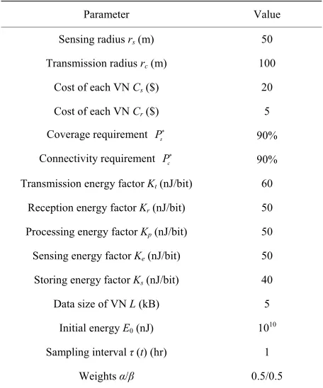
Table 1. Parameters for a wireless visual sensor network.

Parameter Value

Sensing radius rs (m) 50

Transmission radius rc (m) 100

Cost of each VN Cs ($) 20

Cost of each VN Cr ($) 5

Coverage requirement Ps



90%

Connectivity requirement P_c

90%

Transmission energy factor Kt (nJ/bit) 60

Reception energy factor Kr (nJ/bit) 50

Processing energy factor Kp (nJ/bit) 50

Sensing energy factor Ke (nJ/bit) 50

Storing energy factor Ks (nJ/bit) 40

Data size of VN L (kB) 5

Initi J)

Sa r)

0

al energy E0 (n 1010

mpling interval τ (t) (h 1

Weights α/β .5/0.5

objectives equally in uation.

To gua omparing the pe rmance,

we con n he following er: for

different re R, we calculate the optimal

numbe f s N and tie aussian

dist proposed deployment

strate e T of VSN are evalu-

ated r comparis rpose,

we f ount to uniformly ran-

dom ted VSN and en com-

pare lifetim under the sam budget.

Next, e uniform an ussian

distributi deployment scheme when

the lifetim maintained at certain period.

For unifor ted VSN, VNs are u iformly

and ind the monitored gion and

are responsib lection and for g. For

ventional o ussian distributed V Ns are d they would take

estment. For limited budget, our pr

urs, 605 hours, and 19

our eval

rantee fairness in c rfo

duct our analysis i t mann

gions with radius

r of VNs M, number o RN r-2 G ribution deviation σ for our

gy. Next, cost C and lifetim

for our proposed strategy. Fo on pu irst utilize the same cost am

VSN and Gaussian distribu e for three strategies

th e we compare the cost of th d Ga

on to our proposed e of the network is

m random distribu n

ependently deployed in re

le for data col ne-tier Ga

wardin SN, V con

deployed as Gaussian distribution an

[image:12.595.310.538.530.705.2]

care of both data collection and forwarding. In the evaluation, we would search optimal Gaussian parameters to guarantee the performance of one-tier Gaussian distribution strategy. We compare three strategies for Circular VSN with radius R = 500 m, 800 m, 1000 m, 1500 m respectively.

Figure 10 shows the lifetime of VSN in different

monitored region using three strategies. We first imple- ment our proposed scheme to optimize deployment parameters for a two-tier VSN. Then, we compute the total

cost of our deployment cost C for four regions and invest the same cost to deploy VNs with two other existing strategies into the same region. From Figure 10, due to

energy-hole problem and cost budget, we can clearly see that in all three strategies, VSN lifetime decreases as area of monitored region increases, which verifies the cor- rectness of our analytical method.

Figure 10 also shows that, as compared to existing

strategies, our proposed scheme always has the best lifetime performance with the same cost for a given area. Using R = 500 m as an example, our proposed two-tier strategy can achieve 1250 hours VSN lifetime with cost $8975. But, uniform strategy VSN can only last 89 hours and conventional Gaussian VSN can reach to 200 hours with the same cost inv

oposed two-tier VSN has 190 hours lifetime in a largearea R = 1500 m, but still beats 14 hours for uniform VSN and 37 hours for conventional Gaussian VSN.

To verify the usefulness of our proposed strategy in cost saving aspect, we also calculate the cost of three strategies when the lifetime of VSN must be maintained as certain hours. We calculate the cost of four different regions with radius R = 500 m, 800 m, 1000 m, 1500 m, respectively. Based on the results of lifetime analysis above, we compare three schemes cost when the lifetime is maintained as 1250 hours, 1249 ho

0 hours for four different regions.

As shown in Figure 11, the total budget of our pro-

posed two-tier VSN is $8975, $35,720, $50,000 and $100,000 for four different regions. The cost of uniform VSN is $125,680, $610,520, $769,440 and $1,327,800, respectively. Cost of a uniform VSN increase dramatically when the region area get larger. One-tier Gaussian strategy costs $22,040, $107,480, $144,680 and $275,620 for four analyzed regions. Its performance on cost aspect is better than a uniform VSN, which is already shown in

(13)

[image:13.595.307.539.83.260.2]

Figure 11. Cost comparison of two strategies with differen

many previous related work, but still worse than our proposed two-tier strategy. The analysis illustrates that no matter what the objective is, lifetime or cost, our proposed two-tier VSN deployment optimization strategy is observed to provide a better performance than a com- monly distributed deployment strategy.

6.2. Optimal deployment Strategy for Elliptical VSN

Suppose we have a two-tier Elliptical VSN with M VNs and N RNs, which is divided into multiple annuli. Similar to Circular VSN, we can model the deployment strategy optimization problem as Equation (38). But, the difference is that we need to search for four deployment parameters M, N, σx, and σy, since σx≠ σy. Although more parameters need to be optimized, brute-force search al

sented for Elliptical VSN

hus,

t region radius for Circular VSN.

- gorithm still works for Elliptical VSN. Search algorithm described in Algorithm 1 is pre

deployment strategy optimization.

Similar to a Circular VSN, the search space could be decided. Mmax and Nmax could be fixed based on the cost budget. Large values of x_max and ymax might cause

unnecessary additional cost, since RNs might be deployed outside the monitored region. T _x_max and

max

y

 could be obtained in the way similar t rcular n σ an d CDF when an Elliptical VSN is modeled as

o Ci VSN scenario. Figure 12 shows us the relation betwee

d σ an

x y

[image:13.595.58.288.84.272.2]

an ellipse with major axes is 1000 m and minor axes is 800 m. CDF at Z axis indicates the percent of RNs within the monitored area. For example, when σx = 600 and σy = 400, there are around 75% RNs are within region boundary and about 25% are wasted, then we can set _x_max = 600 and ymax 400 if the threshold of 75% is accept-

Figure 12. Analysis of maximal range of σx, σy.

able for monitored task. Now, we have the searc ace for Ellipti timization. Algorithm 2 is presented

h sp cal VSN op

for optimization procedure, and computational complex-ity is discussed in Lemma 2.

Lemma 2.Algorithm 2 has a polynomial time com-

putational complexity.

Proof. Same as Algorithm 1, Algorithm 2 also use

brute-force search method to find global optimal results for circular VSN, but searching need to be done for four parameters since σx ≠ σy. Searching space for four parameters M, N, σx, σy are [1, Mmax], [1, Nmax], [1, x_max],

and [1, y_max] respectively.

Searching of optimal number of VNs Mopt in sensing network still cost O(Mmax) computing complexity. In searching optimal parameters for a relay network, for each annulus of VSN, an adaptive recursive Simpson’s algorithm is needed to calculate the lifetime of VSN.

Assum rsive

impson’s algorithm is O(L ) and complexity of ing that complexity of the adaptive recu

S simpson

VSN cost computing is O(C). Then, O(k ×Lsimpson + C) complexity for different N and σx, σy is needed. Therefore, complexity of algorithm 1 is O(Nmax × x_max × ymax ×

(k × Lsimpson + C) + Mmax). Based on the analysis in Lemma 1, we finally have complexity of Algorithm 1

represented as O(Nmax × x_max × ymax × k), which in-

dicates that Algorithm 1 is a polynomial time computa-

tional complexity searching method.

With Algorithm 2 the performance of our proposed

deployment strategy is evaluated. Analysis param rs are also wn in Table 1. F

pare our posed strategy to

ete

sho or Elliptical VSN, we com-

pro uniform and Gaussian de-

ployment strategies for different elliptical region, with major axes a and minor axes b are (a = 400, b = 200), (a

(14)

Input: a, b, rc, rs, α, β, E0, Ps

_,

c

P_,_M

max, Nmax, x_max, ymax, Cs, Cr Output:Mopt, Nopt, x_opt, yopt

forM = 1 Mmaxdo

ifCoverage (a, b, rs) ≥ Ps

 then

M = Mopt

end if end for

for N = 1 Nmaxdo for x = 1 xmax do

for y = 1  ymax do ifConnectivity (a, b, rc) ≥ Pc

 then

T = Lifetime (a, b, rc, E0, Mopt); C = Cost (a, b, Mopt); W = αlnT – βlnC;

if W > Wmax & x > y then

Nopt = N;

opt

x

 = x;

opt

y

 = _y;

end if end if end for end for end for

Function Coverage (a, b, rs) Compute Ps with Equation (15);

returnPs;

Function Connectivity (a, b, rc) Compute Pc with Equation (30);

returnPc;

Function Lifetime (a, b, rc, E0, Mopt)

Compute r

i

T, i 1,k with Equation (34); Compute , with Equation (31);

T = min (Ts_, Ts

r i

T), i 1,k;

returnT;

Function Cost (Cm, Cn, Mopt) C = CmMopt + CnN;

[image:14.595.63.294.79.540.2]

returnC;

Figure 13. Lifetime comparison of two strategies with dif-ferent region radius fo Er lliptical VSN.

Figur on of two strategies with different

region liptical VSN.

hours, 663 hours, and 588 hours in ur sample region. The costs of VSN in four monitored

e it

e 14. Cost radius for El

comparis

for 1250 hours, 841 Algorithm 2. Global optimal parameters search algorithm

for a Elliptical VSN.

three strategies VSN. Similar to Circular VSN analysis, we optimize the lifetime of VSN with cost $1915, $3465, $5860 and $8990. Then, with the same amount, we test that a uniform distribution strategy has the worst lifetime performance and optimized conventional one-tier Gaus- sian strategy lifetime performance is still worse than our proposed idea. For scenario in our analysis with parameters in Table 1, our two-tier strategy would prolong the

lifetime of VSN by at least 6 times with the same cost. After comparison of VSN lifetime, cost of VSN for maintaining certain period lifetime is analyzed in Figure 14. Continuing from the results of our earlier analysis,

lifetime of VSN with our two-tier strategy are optimized fo

region using three strategies are shown in Figure 14. We

note that our proposed strategy always shows smallest cost for VSN to maintain certain lifetime period and is able to keep the VSN cost increase slower than other two strategies when monitored region is increased. The uniform strategy normally needs the largest cost and cost increases quickly when the area of monitored region is increased. Gaussian strategy has a better performance in term of the cost than a uniform method. However, sinc

only deploys VNs, cost is wasted on extra VNs, which only provide packets forwarding function and camera hardware are not used.

[image:14.595.311.538.82.274.2]