Online Full Text

Abstract - Most studies related to the schedule in

manufacturing system have been focused on developing the algorithm for the single objective of improving unit time productivity by reducing cycle time. That is to build the accurate scheduling by applying various dispatching rules in real-time. This study is focused on the manufacturing process of PR (Photo Resist), one of the material for the FPD (Flat Panel Display) and semi-conduct process. The current system in a practical case is analyzed by simulation. The alternative is suggested to reduce inventory cost and validated by simulation. The suggested simulation experiment will offer the decision variables required for achieve the system objective.

Index Terms— Dispatching rule, Robust Design,

Simulation

I. INTRODUCTION

S manufacturing industry becomes more competitive, the accuracy of order is lower because lead-time decreases, and the time for the primary customer to response to the secondary customer. To solve this problem, CPFR (Collaborative Planning, Forecasting and Replenishment) or VMI (Vendor Managed Inventory) has been studied sharing information between customers and suppliers and building strategies. CPFR or VMI is one of the techniques to reflect supply chain information in manufacturing plan, establish Win-Win relationship between customers and suppliers, and reduce inventory level. However, there are risks of drop in product price and increase in inventory level when the production plan suggested by customer is unreliable or order confirmation period is broken. The situation is worse in customer-oriented market because the influence of suppliers is less than that of customers and it is hard to control the customer orders. So, we suggest the scheduling technique and process redesign

to find the way to reduce inventory cost without any new investment in terms of suppliers. Also, the proposed model is applied to a real business and validated in terms of the effect of the model by concerning inventory cost.

II. LITERATURE REVIEW

Various scheduling methods have been studied to reduce make-span and increase productivity. Lu, et al, Kumar, Li, et al. (1996) and Lin, et al. (2001) presented that a suitable dispatching rule is also important to improve system output. Lin, et al. (2001) simulated the dispatching rule method and principle for material handling system in wafer fabrication. They validated that the shortest path to transport equipment and FIFO (First-In First-Out) rule are better than other dispatching rules by representing the dispatching rule, evenly affecting utilization of transport equipment, process of material, waiting time, and average transport time. However, their research only focused on the dispatching rule for transportation system, rather than the dispatching rule for machines. Chen, et al. (2004) suggested a dynamic state-dependent dispatching (DSDD) heuristic method. They developed DSDD considering the state of production system. They identified bottlenecks from the workstations over time, and then, applied three different dispatching rules considering the waiting. And, they demonstrated that DSDD heuristic is preferable to other dispatching rules in terms of average and standard deviation of cycle time and work-in-process. Chan, et al. (2003) developed a dynamic scheduling algorithm for a flexible manufacturing system with pre-emptive approach. They proved that a dynamic scheduling algorithm could improve the system’s performance by experimenting three cases: the system with a broken machine, the system without any broken machine, and the system with a broken machine and biased performance. Chen, et al. (2004) suggested a dynamic state-dependent dispatching (DSDD) heuristic method. They developed DSDD considering the state of production system. They identified bottlenecks from the workstations over time, and then, applied three different dispatching rules considering the waiting. And, they demonstrated that DSDD heuristic is preferable to other dispatching rules in terms of average and standard deviation of cycle time and work-in-process. Sheen, Liao, and Lin (2008) developed a branch and bound algorithm with the different capability of machines because of machine breakdown or other unavoidable reasons. The algorithm included the availability and eligibility of machines in the parallel machine scheduling. They proved that the proposed algorithm can reach the optimal solution for the instances minimizing the maximum lateness.

A Simulation Study on Development of

Scheduling for Reducing Cost

Using Robust Design

Kwang MoYang, Jong Hyun Jo, Sung Hee Choi, Sung Woo Kang , Seung Hun La , Kyong Sik Kang

A

Manuscript received December 06, 2010; revised January 21, 2011. Kwang MoYang is with Department of Industrial Engineering, Yuhan University, South Korea (corresponding author; phone: 82-2-2610-0755; fax: 82-2-2615-6614; email: [email protected]).

Jong Hyun Jo is a Ph.D student in Department of Industrial & Management Engineering, Myongji University, South Korea ([email protected]).

Sung Hee Choi is a Ph. D student in Harold and Inge Marcus Department of Industrial and Manufacturing Engineering, Pennsylvania State University, U.S. (email: [email protected]).

Sung Woo Kang is a Ph. D student in Harold and Inge Marcus Department of Industrial and Manufacturing Engineering, Pennsylvania State University, U.S. (email: [email protected]).

Seung Hun La is with Department of Industrial and System Management, Myongji College, South Korea (email: [email protected]).

machines, few is studied on the scheduling research product family under various manufacturing conditions for by as yet. Also, most dispatching rule for wafer fabrication process is simple FCFS (First-Come First-Serve) with a single objective. The main aim of this research is to simulate and validated the effect of the accurate schedule for the wafer fabrication system to meet the business purpose and decrease inventory cost.

III. THE CURRENT SYSTEM ANALYSIS

A. The system analysis for simulation analysis

The real business is a manufacturing company to produce PR (Photo Resist) and the related for flat panel displays and semi-conduct products. The faced problems of this business are the same as above the problems of material handling system in wafer fabrication.

Since the business is a kind of equipment industries based on machinery and concerns investments on the facilities, it could not afford to increase capacity. Also, it is hard to fix the order confirmation period because of modification of orders. Since large part of raw materials relies on imported materials, a great change in order is disallowed, and, especially, it is disabling to cancel the order after shipping the materials. For that reason, the suppliers should suffer high inventory level and the additional inventory for backlog due to the short deadline. Figure 3.1 describes the process layout of the company for our case study.

Melting and stirring stage is for melting the raw material with even solubility. After that, the melted raw materials is measured according to BOM and sent to a mixing tank with a certain rate for a product. The materials in the mixing tank are mixed evenly in the mixing stage. The mixed product is screened to meet the customer needs in the filtering stage and packed to ship. The scope of this paper is form the melting and stirring to filtering stage, and the package stage is excluded in this paper. The numbers of machines for each stage and the operational rate are summarized in Table 3.1, and setup time and run time are described in Table 3.2. The information from Fig. 3.1, Table 3.1, and Table 3.2 is used for simulate the process.

The assumptions for simulation are following:

(1) According to the order, the raw materials are input in

the process without any failure

(2) The working invoice accepted is issued on the

accepted date

(3) The raw material is purchased in proportion to

monthly production, and the beginning inventory of the raw material is zero

(4) There is no actual work-in-process due to many

identical machines although there is some work-in-process because of working delay or machine failure

(5) There is no machine replacement, and the setup time

for changing tank, measurement or filter is negligible because those times are relatively very small to actual processing time. So, the setup times are regarded as the same as the time described in Table 3.2. Since most process is automated, there is no labor shortage for changing product, and there is 2 shift and 16 hours

(6) The maximum capacity of tank is 1,500 L

(7) This model is deterministic

On the assumptions, the most interesting feature is that every process is identical and that there is no replacement. The maximum capacity per lot is 1,500L because the capacity of tank is 1,500L.

B. The simulation analysis for the current system

In this study, the simulation models for both the current system and the suggested system are built to validate the effect of the proposed system by Rockwell ARENA 7.0. The model is described the result is summarized in Table 3.3.

TABLE3.2.

THE SETUP TIME AND RUN TIME FOR EACH PROCESS AND PRODUCT

Process

No. Process

Run Time (Hour) PR-1 PR-2 PR-3 PR-4 PR-5 PR-6 10

Melting and Stirring

5 3 3.5 18 15 17 20 Measuring 0.5 0.5 0.5 0.5 0.5 0.5 30 Mixing 5 5 5 32 31 32 40 Filtering 4 3.5 4 4 4 3.5

TABLE3.1

THE NUMBER OF FACILITIES FOR EACH PROCESS Process

No. Process Facility The number

of facility 10 Melting and

Stirring Mixing Tank 6 20 Measuring Load Cell 3 30 Mixing Composite Mixing

Tank 5

40 Filtering Filter 3

The current system is reflected in the simulation model based on the Table 3.3. In the following section, we derived an alternative to reduce inventory cost by design of experiment. The simulation model presented previously is to result in the optimal solution and validate the reliability of the solution for analyzing the suggested alternative combination.

IV. SIMULATION MODEL

A. Alternative selection

Once the materials for all products input in the production line, the materials go through all processes, such as melting and stirring, measuring, mixing and filtering in the orderly manner, without any work-in-process. Besides, the setup time for changing product is negligible because the setup time is relatively very small than the process time.

To solve the problem the company concerned, we considered EDD, SPT, and LPT for dispatching rule, output, total processing time, and the similarity between inputs for routing module, and forwarding, backwarding and middle for scheduling techniques, as described in Table 4.1. We performed the simulation by combining those alternatives.

B. Design of experiment

the optimal combination. Taguchi technique is employed to design and simulate the combinations.

For factor A, the dispatching rule can be changeable by Queue module in ARENA 7.0. The level 1 for factor B is to group the facilities according to the rate of order/plan, production, and output. According to Table 3.3 and 3.4, the total production is 248,000 kg, and the planed output is 195,000 kg. Thus, the rate of the planed output is approximately 79%. Grouping facilities by the production is summarized in Figure 4.1.

For the level 2 of B factor, the facilities are classified according to the total production time for each product. The production time for each product is summarized in Table 4.5.

TABLE4.5

THE TOTAL PRODUCTION TIME FOR EACH PRODUCT Product Total Production time

PR-1 290.0 PR-2 493.0 PR-3 638.0 PR-4 449.5

Fig.4.1. The production process layout for the level 1 of factor B TABLE4.4

THE PRODUCTIONS PLANED AND ORDERED

Section Production Rate Planed 195,000 79% Ordered 53,000 21% Total 248,000 100%

TABLE4.2 THE LEVELS FOR EACH FACTOR Factor Level 1 Level 2 Level 3

A EDD SPT LPT

B Order/Plan Process time Affinity between materials C Forward Backward Middle

TABLE4.1 ALTERNATIVES

Factor Level Detail

A

1 EDD (Earliest Due Date) 2 SPT (Shortest Processing Time) 3 LPT (Largest Processing Time)

B 1

Module by production plan or MTO (Make-To-Order) and the specific routing for the module

2

Module by total processing time for each product and the specific routing for the module

3 Module by similarity between the inputs and the specific routing for the module

C

1 Forward Scheduling 2 Backward Scheduling 3 Middle Scheduling

TABLE3.3.

THE COMPARISON BETWEEN THE CURRENT SYSTEM AND THE

SUGGESTED MODEL

Current system Simulation result

ADDITIVE 318 316 CATALYST 17 17 MONOMER 13 12

PAC 2,090 2,085

RESIN 9,717 9,716

SOLVENT 76,630 76,623

SURFACTANT 72 70 Total cost

In Table 4.5 the products can be classified into two groups, such as product PR-1, PR-5, and PR-6 and PR-2, PR-3, and PR-4 based on 400 hours. The total production time for all products is 2,465 hours, and the total production time for the PR-1, PR-5, and PR-6 group is 1,580.5 hours, 64% of the total production time for all products. For the level 3 of factor F, the facilities are classified by common material and output. The product 2, 4, 5, and PR-6 are classified in the same group because they require the same materials, and the rest two products are in the same group. The total output for all products is 248,000kg, and the total output for the product PR-2, PR-4, PR-5, and PR-6 is 155,000kg and 63% of the total output for all products.

Factor C is related to scheduling, developed to 3 levels and depicted in Figure 4.3

Using Create Module in ARENA 7.0 can change the design for simulation.

The table of orthogonal arrays is built by using Taguchi tool in Minitab R14 to perform the experiment for each alternative. The experiment is repeated 10 times for each combination. The results of the experiment are represented by the quantity of inventory for each material and the inventory cost for the total materials. Since the smaller inventory and cost, the better, the result is analyzed in terms of the smaller-the-better characteristics.

V. THE SIMULATION AND ANALYSIS

A. Simulation analysis

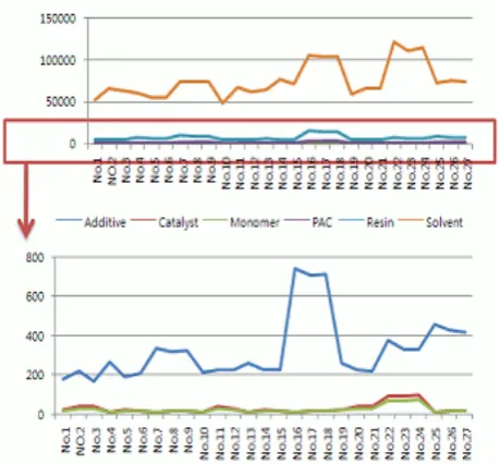
The simulation is performed based on the Table 4.7, and the result is summarized by materials, such as Additive, Catalyst, Monomer, PAC, Resin, Solvent, and Surfactant. The results are depicted in Figure 5.1.

B. The result analysis for cost and validation 1) The result analysis for cost

Considering the simulation result, the optimal alternative is different according to materials. It is hard to identify which alternative is the best, and it is possible to dramatically increase the total inventory cost when an alternative is chosen for the optimum for a certain material. For that reason, the optimal alternative is determined by the unit cost for each material, the material quantities derived from the experiment. The formula to calculate the total inventory cost is expressed in formula 1.

MQ : The inventory quantity for material j of product i

MCij : The unit cost of material j for product i

y ∑ni 1∑mj 1MQ_ij MCij (1)

To compare the difference between the current system and the suggested system, the results for current system and those for the suggested system are summarized in Table 5.1.

Fig. 5.1. The simulation result of the cost for each material

Fig. 4.3. The used scheduling methods for factor C TABLE4.6

THE OUTPUT FOR EACH GROUP BY COMMON MATERIALS

Group Output Ratio

Based on the simulation result in Table 5.1, the combination of A2B1C1 expenses the smallest inventory cost.

2) The validation

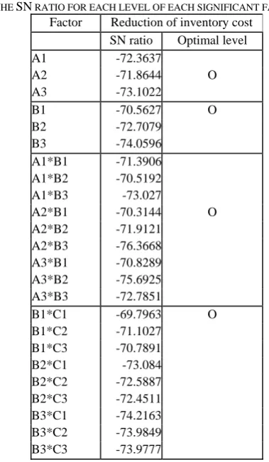
To validate the simulation and robust design, ANOVA (Analysis of variance), the main effect for each factor, and the SN ration for interaction are measured. In terms of the total inventory cost, the statistical significance for each alternative is tested by ANOVA, and the result is summarized in Table 5.2.

According to the Table 5.2, the alternative C is not significant because the p-value is larger than 0.05. While, the differences between levels are statistically significant since the p-values are less than 0.05. The interactions between dispatching rule and scheduling and between facility group and scheduling are statistically significant with 0.05 of significant level. That is, cost can decrease according to the levels of factor A and B. The SN ratio is calculated considering the significant factor and interactions for the inventory cost, and the results are summarized in Table 5.3.

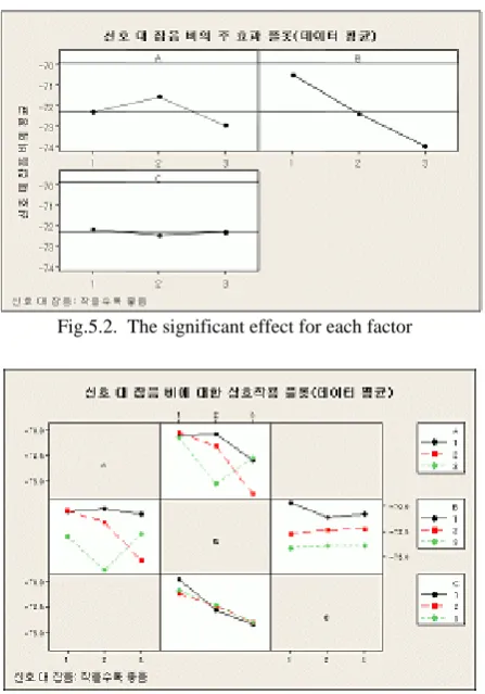
The significant effect and interaction effect for each factor is analyzed using Minitab R14 and illustrated in Figure 5.2 and Figure 5.3.

TABLE 5. 3

THE SN RATIO FOR EACH LEVEL OF EACH SIGNIFICANT FACTOR Factor Reduction of inventory cost

SN ratio Optimal level A1 -72.3637

A2 -71.8644 O

A3 -73.1022

B1 -70.5627 O

B2 -72.7079 B3 -74.0596 A1*B1 -71.3906 A1*B2 -70.5192 A1*B3 -73.027

A2*B1 -70.3144 O

A2*B2 -71.9121 A2*B3 -76.3668 A3*B1 -70.8289 A3*B2 -75.6925 A3*B3 -72.7851

B1*C1 -69.7963 O

B1*C2 -71.1027 B1*C3 -70.7891 B2*C1 -73.084 B2*C2 -72.5887 B2*C3 -72.4511

B3*C1 -74.2163 B3*C2 -73.9849 B3*C3 -73.9777

TABLE 5.2

THE ANOVA TEST RESULT FOR THE TOTAL INVENTORY COST Source DF SS MS F P

A 2 4,252,742 2,126,371 55.98 0.000 B 2 14,016,094 7,008,047 184.49 0.000 C 2 15,827 7,914 0.21 0.816 A*B 4 16,336,039 4,084,010 107.51 0.000 A*C 4 191,789 47,947 1.26 0.360 B*C 4 644,276 161,069 4.24 0.039 Error 8 303,887 37,986

Total 26 35,760,654 TABLE 5.1

THE COMPARISON BETWEEN THE CURRENT SYSTEM AND THE

SIMULATION RESULT

No.

Alternative Repeat

Average SN ratio A B C 1 2 3 4 5 6 7 8 9 10

The current system 5,246 4,152 3,996 4,542 5,011 4,699 4,777 4,855 3,996 4,933 4,621 -73.33

1 1 1 1 3,763 2,503 3,011 2,748 3,102 2,501 3,345 3,939 2,250 3,352 3,051 -69.82

2 1 1 2 3,658 3,574 3,574 3,574 3,403 3,658 3,660 3,570 3,318 3,572 3,556 -71.02

3 1 1 3 3,892 3,569 3,244 3,816 3,814 3,044 3,753 3,723 2,724 2,802 3,438 -70.79

4 1 2 1 4,115 2,835 3,531 2,908 3,609 3,002 4,213 5,255 3,350 3,531 3,635 -71.37

5 1 2 2 3,585 2,759 2,691 3,605 3,700 2,956 3,761 3,317 2,859 2,441 3,167 -70.10

6 1 2 3 3,800 2,775 3,040 3,507 3,155 2,970 3,799 3,020 2,872 2,789 3,173 -70.09

7 1 3 1 5,387 4,196 4,274 4,118 4,977 4,118 5,212 5,212 3,409 4,665 4,557 -73.25

8 1 3 2 4,602 4,427 4,192 4,583 4,192 4,349 4,974 3,958 4,427 4,192 4,390 -72.86

9 1 3 3 4,739 4,427 4,114 4,583 4,349 4,270 4,974 4,192 4,583 4,192 4,442 -72.97

10 2 1 1 3,358 2,573 2,432 3,057 2,745 2,472 2,683 3,406 2,180 3,060 2,797 -69.02

11 2 1 2 3,660 3,660 3,660 3,660 3,660 3,660 3,660 3,660 3,660 3,660 3,660 -71.27

12 2 1 3 3,660 2,963 2,884 3,427 3,660 2,963 3,660 4,104 2,884 3,660 3,387 -70.66

13 2 2 1 3,122 3,062 2,788 3,911 4,396 3,206 3,206 6,717 2,788 2,955 3,615 -71.57

14 2 2 2 4,551 4,095 3,448 3,298 4,896 3,211 6,058 5,241 2,502 2,920 4,022 -72.39

15 2 2 3 5,297 3,043 2,793 3,508 4,467 3,211 4,467 5,152 2,960 2,709 3,761 -71.77

16 2 3 1 7,195 6,450 6,853 6,528 6,684 6,372 7,020 6,853 6,684 6,944 6,758 -76.60

17 2 3 2 6,370 6,212 6,370 6,607 5,977 6,528 6,858 7,040 6,212 6,528 6,470 -76.23

18 2 3 3 6,778 6,213 6,292 6,607 5,901 6,607 6,607 7,389 6,368 6,212 6,497 -76.27

19 3 1 1 3,792 2,461 2,741 4,278 3,051 2,473 3,715 4,211 2,838 3,514 3,307 -70.55

20 3 1 2 3,597 3,580 3,420 3,757 3,500 3,420 3,580 3,597 3,500 3,580 3,553 -71.02

21 3 1 3 3,518 3,580 3,420 3,677 3,500 3,500 3,420 3,597 3,340 3,580 3,513 -70.92

22 3 2 1 7,689 3,550 7,772 6,746 5,371 3,550 8,023 7,809 4,776 7,772 6,306 -76.31

23 3 2 2 6,211 3,890 6,727 7,073 3,871 3,261 6,983 7,319 3,456 6,902 5,569 -75.27

24 3 2 3 5,007 6,818 6,904 6,818 3,867 3,261 7,073 7,152 3,639 6,987 5,753 -75.50

25 3 3 1 4,852 3,918 4,419 4,336 4,503 3,751 4,594 4,930 3,403 4,677 4,338 -72.80

26 3 3 2 4,774 4,428 3,641 5,012 4,781 3,919 4,672 4,519 3,836 4,164 4,375 -72.86

According to the Figure 5.2 and 5.3, the optimal

combination is A2B1C1 which means the inventory cost is

minimum when dispatching rule is SPT, facilities are classified into planed produce and ordered produce, and scheduling method is forward scheduling. The result is consistent with that the average inventory cost of alternative

A2B1C1is the minimum. In terms of SN ratio for each

alternative, the ratio indicates A2B1C1 is the optimal

alternative. To sum up, the total inventory cost could be

changed from ￦ 4,621,000,000 to 2,797,000,000 when the

current system consisting of FCFS dispatching rule FCFS of the current dispatching rule without facility module is changed to the suggested system composed of SPT dispatching rule, planed and ordered production module, and forward scheduling. With the suggested system the output for each product is different, and the differences are summarized in Table 5.4.

VI. CONCLUSION AND FURTHER STUDY

This study assumed that the efficient scheduling and the reduction of inventory are prior for a manufacturing business to be competitive. Dispatching rule, group technology, derives the alternatives and scheduling, and the combinations of those factors are tested by simulation. The optimal combination is determined by the simulation result based on the Taguchi method. The optimal combination is

￦4,62,000,000 to 2,797,000,000. The optimal alternative

cannot be applied to all electronic manufacturing business. Thus, mixed or weighted dispatching rules are considered in simulation, and more alternatives are derived from more practical cases. The alternatives derived by the suggested method and simulation program reduce the cost and time to search optimal solution for improving processes. This study builds the model to decrease inventory cost. Further, the simulation model should be considered in terms of customer service, delivery, and weight for factor.

REFERENCES

[1] Baek, D.H., Yoon, W.C and Park, S.C. (1998), A spatial rule adaptation procedure for reliable production control in a wafer fabrication system, International Journal of Production, Research 36(6), 1475-1491.

[2] Chan, F.T.S., Chan, H.K., Lau, H.C.W., and Ip, R.W.L. (2003). Analysis of dynamic dispatching rules for a flexible manufacturing system. Journal of Materials Processing Technology, 138(1-3), 325–331

[3] Chen, J. C., Chen, C. W., Tai, C. Y., & Tyan, J. C. (2004). Dynamic state dependent dispatching for wafer fabrication. International Journal of Production Research, 42(21), 4547–4562.

[4] Fernango Marin Martinez & Luis Miguel Arreche Bedia(2002), Modular simulation tool for modeling JIT manufacturing, International Journal of Production Research, 40(7), 1529-1547. [5] Hung, Y. F. and Chen, I. P.(1998), A simulation study of dispatch rules

for reducing flow times in semiconductor wafer fabrication, Production Planning & Control, 9(7), 714-722,

[6] Kamrani, Ali K.(1997), Modular Design Methodology for Complex Parts, Industrial Engineering Research Conference, Miami Beach, Florida, May.

[7] Kamrani, A. K., & Salhieh, S. M. (2000). Product Design for Modularity. Boston: Kluwer Academic Publishers

[8] Khoo, L. P., & Situmdrang, T. D.(2003), Solving the assembly configuration problem for modular products using an immune algorithm approach International Journal of Production Research, 41(15), 3419-3434.

[9] Lin, J, T., Wang, F. and Yen, P.(2001), Simulation analysis of dispatching rules for an automated interbay material handling system in wafer fab, International Journal of Production Research 39(6), 1221-1238.

[10] Lin, J, T., Wang, F. and Yen, P.(2001), "Simulation analysis of dispatching rules for an automated interbay material handling system in wafer fab", International Journal of Production Research 39(6), 1221-1238.

[11] Matzler, K., and Hinterhuber, H. H.(1998), How to Make Product Development Projects More Successful by Integrating Kano's Model of Customer Satisfaction into Quality Function Deployment, Technovation, 18(1), 25-38.

[12] Nakata, T., Matsui, K., Miyake, Y. and Nishioka, K.(1999), Dynamic bottleneck control in wide variety production factory, IEEE Transactions on Semiconductor Manufacturing, 12(3), 273-280. [13] Pinedo(2001), “Scheduling 2/E: Theory, Algorithm, and Systems”,

Prentice Hall.

[14] Sheen, G.J., Liao, L. W. and Lin, C. F. (2008). Optimal parallel machines scheduling with machine availability and eligibility constraints. The International Journal of Advanced Manufacturing Technology, 36(1-2), 132-139.

[15] W. David Kelton, Randall P. Sadowski, Deborah A. Sadowski(2002), Simulation With Arena Second Edition, McGraw Hill.

TABLE 5. 4

THE COMPARISON BETWEEN THE OUTPUT OF THE CURRENT SYSTEM AND THAT OF THE SUGGESTED SYSTEM

Product Output of the current system

Output of the

suggested system Difference PR-1 24,000 28,000 + 4,000 PR-2 45,000 50,000 + 5,000 PR-3 50,000 65,000 + 15,000 PR-4 23,722 14,852 - 8,870 PR-5 25,000 25,000 0 PR-6 4,500 13,000 + 8,500

Total 172,222 195,852 + 23,630