On the Performance of Sequential and Parallel
Algorithm for Solving the Forward Problem of the
Two-Dimensional Impedance Equation
A. Bucio R.
IAENG, Member, A. Hernandez-Becerril
IAENG, Member,
C. M. A. Robles G.
IAENG, Member
and M. P. Ramirez T.
IAENG, Member.
Abstract—We study the performance of the numerical method for solving the forward problem of the two-dimensional Impedance Equation [15]. This numerical method is based upon the elements of the modern Pseudoanalytic Function Theory. Considering divide and conquer technique for constructing the parallel algorithm, some sub process can be taking advantage by processing them independently, we parallelize some processes of the numerical method through CUDA technology, obtaining considerable reduction of the temporal complexity. The pro-cessing time of the posed method is evaluated comparing with its sequential version and the speed-up rate of the parallel algorithm respect to the sequential one posed in [15]. The collection of experiments are displayed for illustrating its effectiveness.
Index Terms—Algorithm, CUDA, Electrical Impedance To-mography, Pseudoanalytic Functions Theory, Parrallel Process-ing, Vekua Equation.
I. INTRODUCTION
T
HE Pseudoanalytic Function Theory [3] has been just found to be an important tool for modern Mathematical Physics, and in sequel, for different branches of Engineering. Perhaps, beyond the original expectations that its main cre-ators, professors L. Bers [3] and I. Vekua [20], could have foreseen at the time they first published the foundations of the theory.The elements of the modern Pseudoanalytic Function Theory [12], have been considered as an important tool in Applied Mathematics and Theoretical Physics (see e.g. [4], [12] and [18]). This tool has been successfully applied for solving the forward problem of the two-dimensional Impedance Equation [15]
div(σgradu) = 0, (1)
whereσis the conductivity anduis the electric potential. It is possible to approach the general solution of (1) in asymptotic form, through the Taylor series in formal powers [3].
The detection of the relation between (1) in the plane, and the Vekua equation [20], by V. Kravchenko [13], and shortly after by K. Astala and L. P¨aiv¨arinta [1], opened a complete new path for constructing numerical solutions of the forward problem corresponding to (1), based upon the modern Pseudoanalytic Function Theory [3].
The most important fact of caring about efficiently solving the forward problem for (1), is to use this problem as
A. Bucio R. is with the National Polytechnique Institute, UPIITA, Mexico, [email protected]
A. Hernandez-Becerril, C. M. A. Robles G. and M. P. Ramirez T.
are with Postgraduate Section of Mechanical Engineering School, Instituto Politecnico Nacional Mexico City, Mexico., [email protected]
an approach to the solution of the Electrical Impedance Tomography Problem (also called inverse problem). This problem was widely exposed in plenty works, among which [21] is one of the most important. In this sense, the results posed in [13], and subsequently rediscovered in [1], are indeed very significant, because they allowed to find out the rink for approaching the general solution of the two-dimensional Impedance Equation.
The main contribution of this work is to analyse the performance of the numerical method and its sequential algorithm posed in [15] versus the parallel algorithm to be presented in this work. Employing this numerical method we propose the design of a parallel algorithm using divide and conquer technique [14] with CUDA technology, this will help us to obtain an adequate balance between the computational cost and accuracy. Then we examine some specific examples, in order to illustrate a comparison of the performance and effectiveness between the sequential and parallel method. The conclusions contain the arguments that justify the viability of employing this numerical method as an approach for employing it in medical image [21] this is for solving the Electrical Impedance Tomography Problem [6]. This work is organized as follows: In the second Section , we will explain the mathematical tools necessaries for the construction of the numerical method and algorithm for the forward problem of the two-dimensional Impedance Equation. In Section 3, we describe both algorithms. Then we will show some experimental results of the implementation of both algorithms employing different conductivity functions and finally the conclusions of this work.
II. ELEMENTS OFPSEUDOANALYTICFUNCTIONTHEORY AND ITS RELATION WITH THEELECTRICALIMPEDANCE
EQUATION.
Let us consider the two-dimensional case of the Electrical Impedance Equation:
div(σgradu) = 0,
whereuis the electric potential andσis a separable-variables non-vanishing function within a bounded domain Ω, with boundaryΓ, such that:
σ=σ1(x)·σ2(y). (2)
Introducing the following notations:
W =√σ∂xu−i
√
σ∂yu, p=
s
σ2(y)
σ1(x)
wherei2=−1,∂
x= ∂x∂ and∂y= ∂y∂ ; the equation (1) can be rewritten and transformed into a Vekua equation [20] of the form:
∂zW − ∂zp
p W = 0, (4)
where ∂z = ∂x +i∂y, and W represents the complex conjugation of W:W =ReW−iImW.
The general solution of the equation (4) can be expressed in terms of the Taylor series in formal powers [3]:
W =
∞
X
n=0
Z(n)(an, z0;z). (5)
This is a generalization of the classical postulates of Complex Analysis, that was mainly developed by L. Bers [3]. The following paragraphs contain a condensed description of the material that will be needed for our further discussions. The reader can find a complete and detailed explanation of these postulates in [3] and [12].
A. Taylor Series in Formal Powers.
The formal power Z0(0)(a0, z0;z) with complex constant
coefficienta0, center atz0, depending uponz, formal
expo-nent0, and corresponding to the generating pair(F0, G0); is
expressed as:
Z0(0)(a0, z0;z) =λ0F0+µ0G0;
whereλ0 andµ0 are real constants such that
λ0F0(z0) +µ0G0(z0) =a0;
and
F0=p, G0=
i p.
whereppossesses the form (3).
The formal powers with higher formal exponents n, are defined by the recursive integral expressions:
Zj(0n)(an, z0;z) =n
Z z
z0
Zj(1n−1)(a0, z0;z)d(Fj0,Gj0)z. (6)
where j0 = 0,1 and j1 = 1,0. This is, if j0 = 0 then
j1= 1, and if j0= 1thenj1= 0. The integral expressions
in the right-hand side of (6) are what can be considered antiderivatives in the sense of Bers [3]:
Z z
z0
Zj(n−1)
1 (a0, z0;z)d(Fj0,Gj0)z=
=Gj0Re
Z
Λ
Fj∗0Z
(n−1)
j1 (a0, z0;z)dz+
+Fj0Re
Z
Λ
G∗j0Zj(n−1)
1 (a0, z0;z)dz.
Here,Λ is a rectifiable curve going fromz0uptoz, and:
F1=
√
σ, G1=
i
√
σ.
whereas
Fj∗
0 =−iFj0, G
∗
j0 =−iGj0,
as well
Fj∗1 =−iFj1, G
∗
j1 =−iGj1.
A detailed description of the construction of the formal powers can be found in [3] and [12]. Here we will only remark the two fundamental properties for this work.
1)
lim
z→z0
Z(n)(an, z0;z) =an(z−z0)n. (7)
2) Let an = a0n +ian00, where a0n and a00n are both real constants. Thus
Z(n)(an, z0;z) =
=a0nZ(n)(1, z0;z) +a00nZ
(n)(i, z
0;z). (8)
The absence of the sub index j0 and j1 indicates that the
properties are valid for all formal powers.
Notice the last statement establishes that any formal power
Z(n)(an, z0;z)can be approached by the linear combination
of Z(n)(1, z
0;z) andZ(n)(i, z0;z), thus the numerical
cal-culations shall be exclusively performed to approach these two classes of formal powers.
On the other hand, in [9] is shown the proof of complete-ness of the set:
n
ReZ(n)(1, z0;z)|Γ,ReZ(n)(i, z0;z)|Γ
o∞
n=0
, (9)
for approaching solutions of the forward Dirichlet boundary value problem corresponding to the equation (1).
This is, given a non-vanishing functionσwithin a bounded domainΩ, with boundaryΓ, any boundary conditionu|Γ can
be approached by the linear combination of the elements belonging to (9), that are the real parts of the formal powers with coefficients1 andi, valued at the points belonging to the boundaryΓ:
u|Γ=
∞
X
n=0
c(1)n ReZ(n)(1, z0;z)|Γ+
+
∞
X
n=0
c(ni)ReZ(n)(i, z0;z)|Γ, (10)
wherec(1)n andc
(i)
n are all real constant coefficients. A final statement is in place before studying the numerical method for approaching the elements of (9).
Employing the conjecture posed in [18], we can analyse a variety of conductivity functions and domains in [17]. This conjecture establishes that any functionσ, fully defined within a domainΩ, can be considered at every single point, a special separable-variables function for whichj0=j1, thus
it can be employed for numerically approaching the elements of (9).
B. Numerical approaching of the formal powers.
with coefficients an = 1, since there is not any important methodological variation when consideringan=i.
Therefore, we will consider a collection of K+ 1points
{r[k]}, k= 0,1, ..., K;
equidistantly located in a closed interval[0,1]. If the interval [0,1] coincides with a radius R of the unit circle, whose center is z0 = 0, with some specific angle θ ∈[0,2π), we
will obtain a collection of points in the plane:
{(x[k], y[k])}, k= 0,1, ...K;
constructed as follows
x[k] =r[k] cos(θ); y[k] =r[k] sin(θ).
The formal powers over such radiusRcan be approached employing the recursive expressions:
Z(n+1)[k] =AF[k]· ·Re
k
X
q=0
G∗[q]Z(n)[q] +G∗[q+ 1]Z(n)[q+ 1]∆z[q]+ +AG[k]·
·Re k
X
q=0
F∗[q]Z(n)[q] +F∗[q+ 1]Z(n)[q+ 1]∆z[q],
(11) where
∆z[q] =x[q+ 1]−x[q] +i(y[q+ 1]−y[q]),
andA is a factor that ensures the numerical stability of the method (for additional information see [5] and [15]).
Hereinafter, for briefness we will denote the operations described in (11) with the following form:
Z(n)[k] =BhZ(n−1)[k]i.
III. DEVELOPMENT OF THEALGORITHMS
In previous works, first in [4] was presented a numerical method for constructing the so-called Taylor Series in formal powers and its application to the two-dimensional case of the electrical impedance equation (1), afterwards in [5] was posed the simplified method for numerically solve equation (1) and finally in [15] was presented the optimized numerical method and its sequential algorithm for solving equation (1). Thus, in this work we will describe the most important characteristics of the algorithm presented in [15] and employ-ing this algorithm as baseline we developed a parallel algo-rithm using CUDA technology. For making a clear descrip-tion of both the sequential [15] and the parallel algorithms, in the next subsections we will summarize the programming details including the pseudo code of the algorithms. For constructing the solution for the forward problem of the two-dimensional impedance equation we employed the following parameters:N formal powers numerically approached, over
S number of radii, and consideringK+ 1points per radius. It is essential to remark that the numerical method was fully developed inC, employing as graphic card an NVIDIA
R
GeForceR GTX 770M GPU, this GPU posses 960 CUDA
cores is important to mention that with the evolution of graphic cards will improve performance of the algorithms including the speed up of memory and number of cores. The processor IntelR CoreTMi7-4700MQ CPU @2.40GHz
2.40GHz.
A. Sequential Algorithm
As a measure of the efficiency of an algorithm, usually are considered the resources consumed by the algorithm, as memory and time. This has been developed to obtain values that specify the evolution of the spending time and memory, that is, depending on the size of the input values. We will describe the algorithm posed in [15], this will give us the values for making a comparison between this sequential algorithm [15] an a new version for parallel processing.
In the Algorithm 1 to handle complex numbers in the nu-merical method detailed in previous Section II, we employed data type struct to manage real and imaginary part. If it observes the Algorithm 1 it can be seen that is conformed by a main process where the Taylor series in formal powers (11) are calculated. Then in function Orthonormalization, we apply the standard Gram-Schmidt Orthonormalization Process for obtaining the following set
{us(l)}2sN=0,
where we obtain a linear independent system of 2N + 1 vectors. After the orthonormalization process, we proceed to approach the solution for the conductivity function σ
within a bounded domainΩ, with boundaryΓ, any boundary conditionu|Γ as shown in equation (10). Finally we save the
results obtained, as the orthogonal system, coefficients and the approach solution.
In order to test out the numerical steadiness and conver-gence of the algorithm we calculate the Lebesgue measure for introducing an error parameterE:
E= Z
Γ
(uc|Γ−uapp)
2
dl
12
. (12)
whereuapprepresents the approached solution. This will help us to compare with other works as [16] and verifying the numerical stability of the algorithms.
B. Parallel Algorithm
About constructing the parallel algorithm for solving the forward problem of the two-dimensional impedance equa-tion we employed divide and conquer technique since is a powerful tool for solving conceptually problems. This technique consist on breaking the problem into sub-problems, and solving the original problem by combining the solution of those sub-problems. This technique is useful for parallel algorithms, because can be adapted for execution in multi-cores, this is, distinct sub-problems can be executed on different cores.
Algorithm 1 Sequential Algorithm for solving the forward problem of the two-dimensional impedance equation
S (Number of radii)
N (Maximum number of Formal Powers)
K+ 1 (Number of points per radius) whiles= 1→S do
whilen= 1→N do whileq= 0→K do
call Coordinates Operations call Conductivities Calculations call Generating Pairs
Z(n)[q] =B
Z(n−1)[q]
end while end while end while
call ORTHONORMALIZATION
call APPROACH BOUNDARY CONDITION
call LEBESGUE MEASURE
saveORTHOGONAL SYSTEM
saveCOEFFICIENTS
function ORTHONORMALIZATION
(Classical Gram-Schmidt Orthonormalization Process) end function
function APPROACH BOUNDARY CONDITION PN
n=0 αnu(n)(1,0, z) +βnu(n)(i,0, z)
end function
function LEBESGUE MEASURE
E=R
Γ(uc|Γ−uapp) 2
dl
1 2
end function
One of the most significant differences between sequential 1 and parallel Algorithm 2 is that for the parallel one we transformed the structs into arrays because while working with CUDA we use arrays that can be easily passed to the device global memory and accessed by each core. And one of the main advantages of this method is that we can greatly increase the parameters employed for the approach, the maximum number of radii and maximum number of points can be raised up to 100,000 this is hard task for the sequential algorithm 1 posed in [15], since the time complexity is high. This advantage not only help us to approximate the solution with a greater convergence but also when considering the possibility of apply this numerical method and algorithm to the solution of the inverse or electrical impedance tomography problem.
IV. EXPERIMENTALRESULTS
We will perform a characterization of the numerical method and algorithms, using as domain the unitary circle, and a variety of conductivity functions. This characterization employs the optimized method, first exposed in [15] and then in [16], using the Pseudoanalytic Function Theory, and taking into account that we can analyse any conductivity function, approaching the solution for the Dirichlet boundary value forward problem.
In this work, we will empathize performance of the time complexity in the sequential and parallel algorithms for comparing its effectiveness with the results obtained in [16] when analysing the unitary disk. We will use conductivity
Algorithm 2 Parallel Algorithm for solving the forward problem of the two-dimensional impedance equation
S (Number of radii)
N (Maximum number of Formal Powers)
K+ 1(Number of points per radius) callNUMERICAL BERS OPERATIONS
callFORMAL POWER APPROACHER
callORTHONORMALIZATION
callAPPROACH BOUNDARY CONDITION
callLEBESGUE MEASURE
saveORTHOGONAL SYSTEM
saveCOEFFICIENTS
functionNUMERICAL BERS OPERATIONS forq= 0→K in parallel do
callCoordinates Operations callConductivities Calculations callGenerating Pairs
end for end in parallel end function
functionFORMAL POWER APPROACHER fors= 1→S do
forn= 1→N do forq= 0→K do
Z(n)[q] =B
Z(n−1)[q]
end for end for end for end function
functionORTHONORMALIZATION
(Classical Gram-Schmidt Orthonormalization Process) end function
functionAPPROACH BOUNDARY CONDITION PN
n=0 αnu(n)(1,0, z) +βnu(n)(i,0, z)
end function
functionLEBESGUE MEASURE
E =RΓ(uc|Γ−uapp)
2
dl
1 2
end function
functions with exact representation, namely, we will exam-ine exponential, Lorentzian and a geometrical distribution constructed with concentric circles.
For this experimental results, we will employ the Algo-rithm 1 and AlgoAlgo-rithm 2 and making variations in the number of formal powersN, number of radiiSand number of points
K will be fixed both in1000.
A. Exponential Conductivity Function Case
Considering a non-separable variables exponential conduc-tivity function with the following form
σ=eαxy, (13)
where α represents a coefficient that is used to change the behaviour of the function, for this case α = 5, this conductivity function is represented in Figure 1. And the boundary condition imposed is given in the next expression:
Fig. 1: Exponential Conductivity Function
TABLE 1: Brief relation of the time complexity in both algorithms with an exponential conductivity function
Formal Powers Time Sequential Time Parallel
N t(seconds) t(seconds)
5 446.3 3.261
10 816.2 3.841
15 1187.342 4.615
20 1567.3 5.391
25 1924.43 6.215
30 2302.0 7.044
35 2688.15 7.794
40 3050.5 8.742
because it is an exact solution of (1), as appointed in [16]. As can be seen in Table 1 the difference in the execution of both algorithms it is remarkable that parallel algorithm has the advantage without loosing accuracy.
B. Lorentzian Conductivity Function Case
For this case we propose a conductivity function with the form:
σ= (x+dx)2+Lc
−1
· (y+dy)2+Lc
−1
, (15)
wheredxanddyrepresent the displacements over thex-axis and y-axis respectively, and Lc denotes a real constant. In Figure 2 is displayed this Lorentzian conductivity function.
We will imposed the boundary condition [18]:
u|Γ =
1
3(x+dx)
3+1
3(y+dy)
3
+Lc(x+dx+y+dy); (16)
since it is an exact solution of (1). In this case we will develop the experiment with Lc = 0.5 and in 2 the results are shown with displacement in axis, but in 3 we displayed
x= 0.5 andy= 0.5.
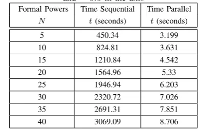
[image:5.595.74.266.231.359.2]In this case we can observe that as it was expected the best results in time complexity are displayed while employing the parallel algorithm. In Table 2 we have no displacement in the conductivity function, but in Table 3 we displacedx= 0.5 and y = 0.5, this cases are important because it can be observed that in Table 3 the time complexity decrease in comparison with the one without displacement since there are more operations that can be executed independently.
Fig. 2: Lorentzian Conductivity Function
TABLE 2: Brief relation of the time complexity in both algorithms with a Lorentzian conductivity function with no displasment in the
axis
Formal Powers Time Sequential Time Parallel
N t(seconds) t(seconds)
5 448.2 3.209
10 813.57 3.59
15 1197.05 4.329
20 1569.81 5.109
25 1943.99 5.992
30 2317.1 6.728
35 2689.09 7.511
40 3026.92 8.35
TABLE 3: Brief relation of the time complexity in both algorithms with a Lorentzian conductivity function with displacementx= 0.5
and= 0.5in the axis
Formal Powers Time Sequential Time Parallel
N t(seconds) t(seconds)
5 450.34 3.199
10 824.81 3.631
15 1210.84 4.542
20 1564.96 5.33
25 1946.94 6.203
30 2320.72 7.026
35 2691.31 7.851
40 3069.09 8.706
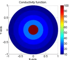
C. Geometrical Conductivity: Concentric Circles
For this case, the conductivity function is composed as follows: one disk with radius r1 = 0.2 representing σ =
100, the ring delimited by r2 = 0.4 and r1 possessing a
conductivity σ = 30, another ring between r3 = 0.6 and
r2 having σ = 20, whereas the one within r4 = 0.8 and
r3 exhibits σ= 15. Finally, the remaining value within the
boundary isσ= 10. The boundary condition is given by the following expression
u|Γ=
1 3(x
3+y3) + 0.5(x+y). (17)
The results are summarized in Table 4.
[image:5.595.334.520.240.365.2] [image:5.595.325.521.411.538.2]Fig. 3: Geometrical conductivity within a non-smooth domain. Combination of a disk and concentric rings.
TABLE 4: Brief relation of the time complexity in both algorithms with a geometrical conductivity distribution constructed with
con-centric circles
Formal Powers Time Sequential Time Parallel
N t(seconds) t(seconds)
5 449.48 3.592
10 825.57 3.918
15 1199.95 4.687
20 1572.79 5.446
25 1928.5 6.061
30 2322.39 7.053
35 2653.13 7.846
40 3001.47 8.746
V. CONCLUSIONS
The construction of the numerical method and algorithms for approaching the solution for the forward problem of the two-dimensional impedance equation, is an important contribution to the Electrical Impedance Tomography theory. This is asserted by considering that the examples presented in this work, could well pose a difficult challenge if analysed with classical numerical methods, as the Finite Element variations are (see e.g. [9]).
In this sense, this numerical method and algorithms can be employed for analysing physical conductivity distributions, since no variations are needed for examining those cases when the exact mathematical expressions are unknown [18]. Furthermore, the results suggest that an adequately balance between the numerical accuracy, steadiness and the compu-tational cost has been achieved. Even though that when using the parallel Algorithm 2 we have as advantage that we can obtain a better approximation to the solution because this algorithm give us the possibility of increasing significantly the parameters of number of points and number of radii. While employing the parallel Algorithm 2 we notice that time complexity reduced considerable, without provoking loss of precision or accuracy. Another important thing that was observed is that the time complexity is proportional to the complexity of the conductivity function.
The development of this parallel algorithm enable us to continue with the hard due of applying this algorithm in the solution of the Electrical Impedance Tomography problem, because this reduction of time will allow us to study more complex conductivity functions and analyse different domains (smooth and non-smooth). When applying this algo-rithm in medical image will be needed to have accuracy with low time complexity. Beside, many characteristics discussed along these pages might be subjects of further works.
Acknowledgements: The authors would like to acknowledge the support of CONACyT.
REFERENCES
[1] K. Astala, L. P¨aiv¨arinta (2006),Calderon’s inverse conductivity problem in the plane, Annals of Mathematics, Vol. 163, pp. 265-299. [2] J. L. Barlow, A. Smoktunowicz, H. Erbay (2005), Improved
Gram-Schmidt Type Downdating Methods, BIT Numerical Mathematics, Vol-ume 45, Issue 2, pp 259-285.
[3] L. Bers (1953),Theory of Pseudoanalytic Functions, IMM, New York University.
[4] A. Bucio R., R. Castillo-Perez, M.P. Ramirez T. (2011), On the Numerical Construction of Formal Powers and their Application to the Electrical Impedance Equation, 8th International Conference on Electrical Engineering, Computing Science and Automatic Control, IEEE Catalog Number: CFP11827-ART, ISBN:978-1-4577-1013-1, pp. 769-774.
[5] A. Bucio R., R. Castillo-Perez, M.P. Ramirez T. and C. M. A. Robles G. (2012),A Simplified Method for Numerically Solving the Impedance Equation in the Plane, 9th International Conference on Electrical Engineering, Computing Science and Automatic Control, IEEE Catalog Number: CFP12827-CDR, ISBN:978-1-4673-2168-6, pp. 225-230. [6] A. P. Calderon (1980),On an inverse boundary value problem, Seminar
on Numerical Analysis and its Applications to Continuum Physics, Soc. Brasil. Mat., pp 65-73.
[7] Z. Cao (2012),New Directions of Modern Cryptography, CRC Press, Shanghai Jiao Tong University, China.
[8] H. M. Campos, R. Castillo-Perez, V. V. Kravchenko (2011), Construc-tion and applicaConstruc-tion of Bergman-type reproducing kernels for boundary and eigenvalue problems in the plane, Complex Variables and Elliptic Equations, 1-38.
[9] R. Castillo-Perez., V. Kravchenko, R. Resendiz V. (2011),Solution of boundary value and eigenvalue problems for second order elliptic op-erators in the plane using pseudoanalytic formal powers, Mathematical Methods in the Applied Sciences, Vol. 34, Issue 4.
[10] S. Kaufhold (Editor) (2013),Proceedings of the XVth International Conference on Electrical Bio-Impedance (ICEBI) and the XIVth Confer-ence on Electrical Impedance Tomography 2013, Heilbad Heiligenstadt, Germany.
[11] Y. Kim, J. G. Webster, W. J. Tompkins (1983),Electrical impedance imaging of the thorax, J Microw Power.
[12] V. V. Kravchenko (2009),Applied Pseudoanalytic Function Theory, Series: Frontiers in Mathematics, ISBN: 978-3-0346-0003-3. [13] V. V. Kravchenko (2005),On the relation of pseudoanalytic function
theory to the two-dimensional stationary Schr¨odinger equation and Taylor series in formal powers for its solutions, Journal of Physics A: Mathematical and General, Vol. 38, No. 18, pp. 3947-3964. [14] Anany V. Levitin, Introduction to the Design and Analysis of
Algo-rithms (Addison Wesley, 2002).
[15] C. M. A Robles G., A. Bucio R., M. P. Ramirez T., (2013),An Opti-mized Numerical Method for Solving the Two-Dimensional Impedance Equation, Proceedings of the World Congress on Engineering and Computer Science 2012 Vol I, ISBN: 978-988-19251-6-9, ISSN: 2078-0958 (Print); ISSN: 2078-0966 (Online).
[16] C. M. A Robles G., A. Bucio R., M. P. Ramirez T., (2013),New Characterization of an Improved Numerical Method for Solving the Electrical Impedance Equation in the Plane: An Approach from the Modern Pseudoanalytic Function Theory, IAENG International Journal of Applied Mathematics, Volume 43, Issue 1.
[17] M. P. Ramirez T., M. C. Robles G., R. A. Hernandez-Becerril (2012),
Study of the forward Dirichlet boundary value problem for the two-dimensional Electrical Impedance Equation, Mathematical Methods in the Applied Sciences (submitted for publication), available in electronic at http://arxiv.org
[18] M. P. Ramirez T., M. C. Robles G., R. A. Hernandez-Becerril, A. Bucio R. (2013),First characterization of a new method for numeri-cally solving the Dirichlet problem of the two-dimensional Electrical Impedance Equation, Journal of Applied Mathematics, Volume 2013, Article ID 493483, 14 pages, Hindawi Publishing Corporation. [19] M. Soleimani (Editor),Proceedings of the 12th International
Confer-ence in Electrical Impedance Tomography, University of Bath, U.K. [20] I. N. Vekua (1962), Generalized Analytic Functions, International
Series of Monographs on Pure and Applied Mathematics, Pergamon Press.