Measuring Dynamic Interaction in Movement Data

Measuring Dynamic Interaction in Movement Data

Jed A. Long1*, Trisalyn A. Nelson1 1

Spatial Pattern Analysis & Research (SPAR) Laboratory Department of Geography, University of Victoria

*Corresponding author email & address:

[email protected]

Department of Geography, University of Victoria PO Box 3060 STN CSC

Victoria, BC V8W 3R4, Canada

Running Head: Measuring Dynamic Interaction

Keywords: dynamic interaction, movement data, correlation, GPS, space-time, local statistics, spatial analysis

Pre-print of published version.

Reference:

Long, JA and TA Nelson. 2013. Measuring dynamic interaction in movement data. Transactions in GIS. 17(1). 62-77.

DOI:

http://dx.doi.org/10.1111/j.1467-9671.2012.01353.x

Disclaimer:

ABSTRACT:

1

The emergence of technologies capable of storing detailed records of object locations has 2

presented scientists and researchers with a wealth of data on object movement. Yet 3

analytical methods for investigating more advanced research questions from such detailed 4

movement datasets remain limited in scope and sophistication. Recent advances in the 5

study of movement data has focused on characterizing types of dynamic interactions, 6

such as single-file motion, while little progress has been made on quantifying the degree 7

of such interactions. In this article, we introduce a new method for measuring dynamic 8

interactions (termed DI) between pairs of moving objects. Simulated movement datasets 9

are used to compare DI with an existing correlation statistic. Two applied examples, team 10

sports and wildlife, are used to further demonstrate the value of the DI approach. The DI

11

method is advantageous in that it measures interaction in both movement direction 12

(termed azimuth) and displacement. As well, the DI approach can be applied at local, 13

interval, episodal, and global levels of analysis. However the DI method is limited to 14

situations where movements of two objects are recorded at simultaneous points in time. 15

In conclusion, DI quantifies the level of dynamic interaction between two moving 16

objects, allowing for more thorough investigation of processes affecting interactive 17

moving objects. 18

1 Introduction

20

The study of individual movement has entered a new era whereby researchers 21

from various fields can benefit from fine resolution object movement data. Technical 22

developments associated with location aware technologies, such as GPS, are transforming 23

representations of movement. Despite improvements in spatially explicit movement 24

datasets, the scope and sophistication of research questions are limited by a lack of 25

methods and analysis (Wolfer et al. 2001). Laube et al. (2007) suggest that within 26

geography, reliance of geographic information systems (GIS) and spatial statistics on 2-27

dimensional representations may be limiting the development of more complex analyses 28

of movement, while disciplines outside of geography may be unaware of the power of 29

spatial (and space-time) analysis. To optimally utilize new movement datasets, analytical 30

techniques capable of addressing more advanced research questions are required. 31

Recently, the identification and measurement of dynamic interactions between 32

moving objects has become an active area of research, likely owing to readily available 33

fine granularity movement data. Dynamic interaction, a term from the wildlife ecology 34

literature, can be defined as the way the movements of two individuals are related 35

(Macdonald et al. 1980) or as inter-dependency in the movements of two individuals 36

(Doncaster 1990). Alternatively, the terms association (Stenhouse et al. 2005), relative 37

motion (Laube et al. 2005), and correlation (Shirabe 2006) have been used to refer to 38

dynamic interactions between moving objects in other examples. All of these terms refer 39

to the same general idea: identifying of how the movements of one individual are related 40

to another. Recent work on dynamic interactions has focused on methods for identifying 41

al. 2010; or chasing behavior, de Lucca Siqueira and Bogorny 2011). However limited 43

work exists on quantifying the strength of dynamic interactions present in movement 44

data. With this in mind we are motivated to investigate methods for measuring the 45

strength of dynamic interactions when there is an expectation that such behavior occurs. 46

This approach differs from recent developments in movement analysis which focus on 47

identifying patterns, defined a priori, from large movement databases. 48

The objective of this work is to extend a previously developed statistic (Shirabe 49

2006) to a measure capable of quantifying the degree of dynamic interaction between 50

moving objects. The new method (termed DI) measures dynamic interaction in 51

coincidental movement segments, that is, it requires movement data of two individuals 52

recorded simultaneously. The DI method is separable into components measuring 53

dynamic interaction in movement direction (azimuth) and movement distance 54

(displacement), termed DIθ and DId respectively. Further, DI is appropriate with the four 55

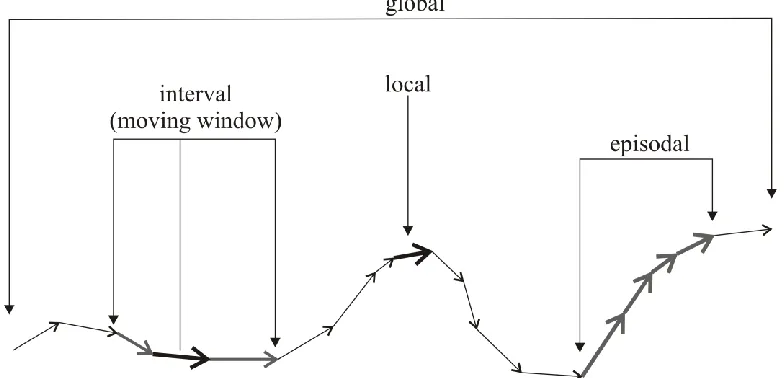
analysis levels (local, interval, episodal, and global – see Figure 1) identified by Laube et 56

al. (2007) with the beneficial property of local values (denoted here using lower-case – 57

di) that aggregate to the interval, episodal and global values. Lastly, DI is derived in a 58

way to allow for a time-lagged approach, but also extensions including time- and 59

distance-based weighting schemes. 60

< Approximate location Figure 1 > 61

2 Related Work

62

This research is motivated by an existing technique (Shirabe 2006) for measuring 63

the strength of dynamic interactions (termed correlations) present in movement data. The 64

of a Pearson product-moment correlation coefficient. Consider two moving objects Ma 66

and Mb, whose spatial coordinates (x, y) are recorded coincidentally at discrete times t = 1 67

… n, termed fixes. Now consider for any M with t = 2…n, V = [Mt – Mt-1] = [vt], is a

68

vector time series of M with n-1 vector segments. A correlation statistic for movement 69

data defined this way takes the form (Shirabe 2006): 70







 









r (1)

71

Where



    1 1 1 1 n t t n v

v are mean coordinate vectors of V. The correlation statistic (r)

72

is defined over the interval [-1, 1] with a score of 1 being perfect positive correlation and 73

a score of -1 perfect negative correlation, with 0 denoting no correlation. 74

The statistic – r, could be advanced in three ways. First, it is dependant on the 75

mean vector of each path, and thus measures correlations in movement deviations from 76

their respective means. The statistic, r, cannot be used for testing direct interactions 77

between two moving objects unless their corresponding mean vectors are identical or 78

near identical. An improved statistic would not rely on this overall mean value. Second, r

79

is unable to disentangle the effects of correlations in movement azimuth and distance, 80

while being sensitive to both. Decomposing such a statistic into components based on 81

movement direction (termed azimuth) and distance (displacement) would be beneficial, 82

as it would allow interactions in these two independent components of movement to be 83

analyzed separately. A third improvement would be a statistic that measures the 84

interaction of each individual movement segment (i.e., local level - Laube et al. 2007). 85

Laube et al. 2007). When movement patterns are characterized by periods of interactive 87

and non-interactive behavior, or varying levels of interactive behavior, a local level 88

statistic will allow a finer treatment of dynamic interactions. 89

Measurements of dynamic interaction in movement data have also been 90

developed by wildlife researchers interested in a finer understanding of wildlife 91

movement processes. The types of interactions studied in wildlife are classified as either 92

static or dynamic interactions (Doncaster 1990; Macdonald et al. 1980). Static interaction 93

relates to how two individuals use space coincidentally, while dynamic interaction 94

reflects how the movements of two individuals are related, for example attraction 95

(Macdonald et al. 1980). Typically, measures of dynamic interaction summarize the 96

proximity of simultaneous movement points. Doncaster (1990) introduced one such 97

measure of dynamic interaction based on the variance/covariance matrix of the spatial 98

coordinates of simultaneous wildlife telemetry fixes; others have used Euclidean distance 99

as an indicator of interaction (Bandeira de Melo et al. 2007; Stenhouse et al. 2005). 100

Stenhouse et al. (2005) further investigated dynamic interaction in grizzly bears (termed 101

associations) by measuring dynamic interaction in movement direction (azimuth – θ) 102

defined as: 103









180 180

   

b

t a

t b

t a t

t ,

f

  

 (2)

104

Equation (2) ranges from 0 –1, with values of 1 when direction of movements is identical 105

and zero when completely opposite (i.e., at 180°). 106

Measuring dynamic interactions in moving object databases is also directly 107

related to a larger body of literature on identifying similar movement trajectories (Sinha 108

commonly employed as a first-step for identifying broader patterns or for detecting 110

clusters in larger movement databases (Benkert et al. 2008; Gao et al. 2010). Moving 111

object pairs that are highly interactive could also be said to follow a similar trajectory in 112

many of these applications, and the methods for detecting dynamic interactions in 113

movement data could be useful for detecting similar movement trajectories. 114

Recently, many new techniques have been developed for categorizing various 115

dynamic interaction patterns commonly found in movement data. Laube et al. (2005) 116

developed a method for detecting RElative MOtion (REMO) classes based upon 117

interpreting patterns of movement direction in groups of moving objects. For example, 118

trend-setting, when one object moves with anticipation of the movement of others, is 119

identifiable using the REMO approach. Noyon et al. (2007) use changes in inter-object 120

distance and velocity to identify relative behavior such as collision avoidance. Benkert et 121

al. (2008) present an algorithm for finding flock patterns in movement databases; which 122

tests whether a group of moving objects are contained in a circle radius r over a given 123

time interval. The study of flocking behavior is useful in the study of wildlife and crowd 124

dynamics (Batty et al. 2003). Buchin et al. (2010) have developed a method for 125

identifying single-file motion in groups of moving objects. Single-file motion is detected 126

using free-space diagrams, derived from the Fréchet distance metric for comparing 127

polygonal curves (Alt and Godau 1995). Related to single-file motion is the detection of 128

chasing behavior, identifiable using the algorithm proposed by de Lucca Siqueira and 129

Bogorny (2011). The methods mentioned above are capable of identifying specific types 130

are unable to quantify the strength of dynamic interactions present, thus motivating the 132

development of quantitative measures of dynamic interaction. 133

3 Derivation

134

In developing a measure of dynamic interaction we consider the rather optimal 135

data situation (as in Shirabe 2006) where two moving objects’ (Ma

and Mb) spatial 136

coordinates (x, y) are recorded coincidentally at discrete times t = 1 … n, termed fixes. 137

For any M with t = 2…n, V = [Mt – Mt-1] = [vt], is a vector time series of M with n-1

138

vector segments. For each movement segment define two fundamental properties: 139

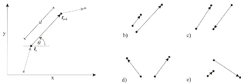
direction (θ), termed azimuth, and length (d), termed displacement. Azimuth (θ) is the 140

angle between a movement segment and a constant axis, most commonly the horizontal 141

axis (Figure 2a). Displacement (d) is the Euclidean distance between two consecutive 142

fixes in a movement segment (Figure 2a). We are interested in deriving a measure of 143

dynamic interaction that separately quantifies interactions in azimuth and displacement 144

(Figure 2b-e). 145

< Approximate location of Figure 2 > 146

3.1 Azimuth – θ 147

To investigate the interaction in movement azimuths we take the cosine of the 148

angle between them. This is simply calculated as: 149









t a t b

t a t

t , cos

f     



θ

di (3)

150

where θt is the angle of movement at time-step t. Here ft has a range of [-1, 1] as desired.

151

The function





t 

 

cos is 1 when movement segments have the same orientation, 0 152

when movement segments are perpendicular, and -1 when in complete opposing 153

directions. In practice if either object (or both) do not move (3) is undefined, because θt is

undefined. Thus, we must consider two alternative scenarios; first if one object moves 155

and one remains stationary, and second if both objects remain stationary. Here we make 156

the assumption that if one moves and the other remains stationary the two objects exhibit 157

no directional interaction, and if both are stationary they are positively interactive. 158

Considering these two alternative scenarios, a complete definition for (3) is: 159









 (4)

160

3.2 Displacement – d 161

Interaction in movement displacement could be measured using a variety of 162

functions. However, it is desirable to have the function (gt) fall in the range of 0 – 1,

163

where a value of 0 represents no interaction and 1 positive interaction. Note there is no 164

consideration of negative interaction in displacement. Using this definition gt can be

165

thought of as a scaling function to ft, and maintains the statistic on the range [-1, 1]. We

166

propose the following function for gt:

167





di (5)

168

Where |·| is the absolute value operator, and α is a scaling parameter defaulting to 1. The 169

function





t d d

g , approaches zero when d_ta >>> d_tb or vice-versa, and is 1 when d_ta =

170

b

t

d . The effect of the scaling parameter (α) on the function g_t





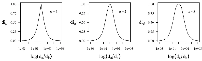
Figure 3. Parameter α can be adjusted to place stricter or looser requirements on 172

similarity in displacement denoting interaction. As α is increased larger differences in 173

reveals that it is undefined when b t a

t d

d  = 0, (i.e., both objects are stationary). If we

175

consider both objects remaining stationary as positive interaction, a more robust 176

definition of (5) is: 177





< Approximate location of Figure 3 > 179

Thus, for two corresponding movement segments, a measure of dynamic 180

interaction is the product between the azimuthal term (ft) and displacement term (gt):

181













t a t t b t a t t b t a

t ,v f , g d ,d

v  _θ  _d    

t di di

di (7)

182

We are motivated to use the functions ft and gt to provide a statistic that covers the range

183

[-1, 1] as was done in Shirabe (2006). Positive values of dit correspond to cohesive or 184

positively interactive movements, while negative values can be interpreted as repulsion or 185

opposing movements. Values near zero should be interpreted as having no interaction. 186

The di statistics measure dynamic interaction based on similarity in azimuth (θ)

187

and displacement (d) of simultaneous movement segments but do not account for the 188

proximity of moving objects. Thus, di represents a similarity index taken in a normalized 189

plane (i.e., the distance between the two objects has no impact on the resulting value). 190

We are motivated to use this type of formulation as the spatial proximity required for 191

dynamic interaction to occur is application specific. It is up to the analyst to decide if two 192

moving objects maintain a requisite proximity for dynamic interaction to occur, then such 193

example when identifying points-of-interest in large movement databases (e.g., Benkert 195

et al. 2007), the di methodshould not be employed. 196

We have made assumptions in the equations for diθ and did regarding how to 197

analyze dynamic interactions when objects do not move (i.e., θ is undefined and d = 0). 198

In certain cases interpretation of these situations will be clear, for example, if one object 199

stops moving, does the other? However in practice, many applications may not facilitate 200

such straight-forward interpretation. For example, when studying urban travelers does 201

stopping at a red-light signify a change to dynamic interaction even if they will 202

eventually go straight? In light of these concerns, these assumptions can be modified to 203

accommodate different situations that may arise in various movement scenarios to fit a 204

given application. 205

3.3 Global analysis 206

A global version of the di statistic can be used to measure the overall interaction 207

in a set of movement segments. First, it is useful to recognize that we can identify global 208

interaction in azimuth or displacement individually by summing the interaction values for 209

each individual segment and dividing by the number of segments. This form of a global 210

DI gives equal weight to each segment. . 211





_

θ V V di

DI (8)

212





_

d V V di

DI (9)

213

A global measure of overall dynamic interaction DI can also be derived. 214





_

_

, di di di

DI V V _{θ d} (10)

It is important to note that in the local version di = diθ × did, but with the global statistic, 216

due to summation rules, DI ≠ DIθ × DId. This can make interpretation of global values of

217

DI less straightforward than with local values. However, if we were to alternatively 218

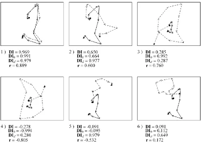
define the global version as DI = DIθ × DId, then the equation defined by (10) would no

219

longer hold. Thus, interpretation of DI values is best done separately for each component 220

(i.e., DI, DIθ, and DId). 221

The global formulation is also appropriate for interval and episodal levels of 222

analysis. Here we simply replace n with some interval or episode length n’, where n’ < n. 223

This type of analysis can be illuminating when analyzing interactions in larger movement 224

datasets, where varying levels of dynamic interaction may occur at different points in the 225

movement paths. 226

3.4 Time- and Distance-based Weighting 227

In instances where the sampling interval of the n fixes is unequal it is desirable to 228

scale the statistic based on the temporal duration of each movement segment. In practice, 229

this would give more weight to segments of longer duration and less weight to shorter 230

segments. Temporal weighting may also be used to account for missing fixes, common to 231

GPS-based tracking data. Let Δt correspond to the temporal duration of segment t, where

232



 

1

1 n

t

t T is the total duration of the entire movement path. Then a time weighted

233

version of (10) is defined as: 234





_



  

1

1 n

t t b

a

T

,V _{θ d}

V di di

DI (11)

235

Viewed in light of the uncertainty associated with movement data, this form of temporal 236

proportional to the duration between fixes; lower weights to segments with higher 238

uncertainty (i.e., more time between fixes) and higher weights to segments with higher 239

certainty or finer space-time resolution. 240

Similarly, we can define a distance-based weighting scheme for (10) where 241

movements with larger displacement have increased weight in calculation of the statistic. 242

Varying distance-based weights could be used when dynamic interactions of a specific 243

movement behavior are of interest. For example in the study of wildlife long directed 244

movements are often interspersed with shorter random movements distinguishing 245

migratory and foraging behavior (Turchin 1998). Distance weighting could be used to 246

tailor the measurement of dynamic interactions to either of migratory or foraging 247

behaviors in this case. A possible distance-based weighting scheme would be the average 248

displacement of two segments: d_tavg 













1

1 n

t avg

t D

d . Based on the

249

average displacement a distance-weighted version of (10) is defined as: 250





_



 

1

1 n

t avg t b

a

D d

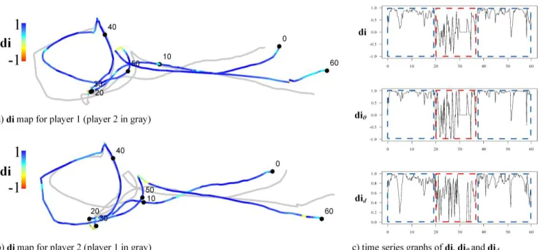
,V _{θ d}

V di di

DI (12)

251

However, the average displacement of two objects movement segments is misleading 252

when one object has a large displacement and the other has a small displacement. Thus, 253

other distance measures are worth investigating for alternative distance-based weighting 254

schemes, keeping in mind that the sum of the weights should equal one. The equations 255

(11) and (12) can be combined to provide a time- and distance-based weighting scheme. 256

It is important to note that time- and distance-based weighting is really only useful when 257

interpreting global results when there is benefit to assigning segments weights based on 258

Another interesting extension to studying correlations in movement paths is when 260

movements interact with a temporal lag, for example when trend-setting occurs, as 261

described by Laube et al. (2005). The DI statistic can be modified to evaluate dynamic 262

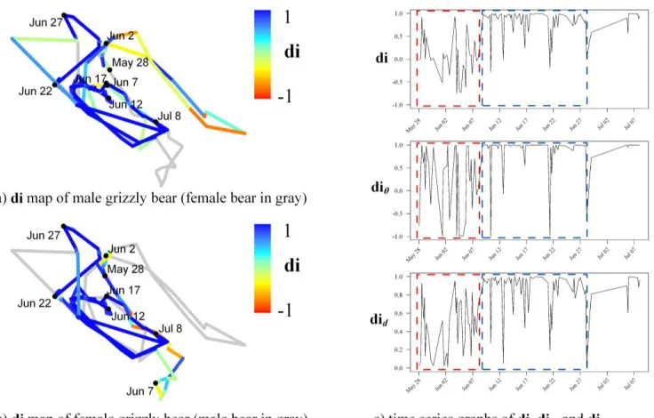
interactions at a temporal lag. To measure dynamic interactions at a temporal lag, select a 263

time lag – k, where k is generally taken to be a multiple of the fix interval (i.e., if fixes are 264

taken at even intervals the time between consecutive fixes). Then we can, alternatively 265

define diθ and did as:

266





k t a t

t ,

f _

  

θ

di (13)

267





k t a t t d ,d

g _



d

di (14)

268

The global statistics (DI, DIθ, DId) can be computed as before, using the time lagged

269

versions of diθ(13) and did (14).

270

4 Data

271

4.1 Simulated Data 272

Six simulated data sets are used to highlight the utility of the DI statistic and the 273

benefit of extensions it makes to r (Shirabe 2006). A single random walk (n = 10) is used 274

to generate a movement path that is the bases for the simulation examples. We used 275

manual permutations to the spatial coordinates of the original random walk to produce 5 276

new movement paths that represent 5 unique dynamic interaction scenarios (Table 1). 277

The first scenario simulates two objects moving with strong-positive dynamic interaction. 278

The second scenario uses the same two paths as the first scenario, but one is rotated at 279

45°, simulating strong interaction in displacement, and low interaction in azimuth. The 280

third scenario simulates positive interaction in azimuth and no interaction in 281

interaction in displacement. The fifth scenario simulates no interaction in azimuth and 283

strong interaction in displacement. The sixth scenario uses a second independent random 284

walk to simulate random interactions between two moving objects. 285

< Approximate location of Table 1 > 286

4.2 Athletes – Ultimate Frisbee 287

In team sports players (objects) movements are expected to be highly interactive. 288

Often a defending player is tasked with “covering” an offensive player, and their 289

movements are in reaction to that offensive player. In the sport of ultimate frisbee, 290

offensive players move about the field in an attempt to get open for a pass from their 291

teammates. Defending players cover them, in an attempt to intercept or dissuade passes 292

from being completed. As such, in ultimate frisbee the movements of an offensive player 293

and their defender are highly interactive. We used 5 Hz sports-specific GPS devices 294

(GPSports, Fyshwick, Australia) to monitor the movements of two ultimate frisbee 295

players over a one minute segment during a training game. In this example, the two 296

players cover each other for the entirety of the one minute period. A total of n = 276 GPS 297

locations (out of a possible 300) were simultaneously recorded. Most of the missing 298

locations occur when the players are relatively stationary. At 5 GPS locations per second 299

this represents an extremely detailed movement dataset, appropriate for investigating the 300

intricate movements of athletes. 301

4.3 Grizzly Bears in Alberta, Canada 302

To further demonstrate DI, we investigate a previously published dataset 303

containing GPS telemetry locations of a number of grizzly bears in Alberta, Canada 304

showed evidence of dynamic interaction during different seasons, in particular male-306

female interactions were strongest during spring when mating activity occurs. To 307

demonstrate DI, we examine one specific male-female bear combination that exhibited a 308

relatively strong association during the mating season (male (G006) and female (G010) - 309

see Fig. 4 in Stenhouse et al. 2005). Grizzly bear GPS collars were programmed to obtain 310

a location fix every four hours, however missing entries are frequent. As a result, only 311

112 simultaneous GPS fixes were obtained for the two bears during period from May 28, 312

2000 to July 08, 2000. In this example, we incorporate time-based weighting in order to 313

account for unevenness in fix intervals (ranging from 4 hours to over 6 days). 314

5 Results

315

5.1 Simulated Data 316

Using the six simulated datasets we compared global values for DI, DIθ, and DId

317

with Shirabe’s (2006) r statistic (Figure 4) to reveal both the similarities and differences 318

between these two methods. In scenario 1, where both movements are highly interactive 319

in both displacement and azimuth, DI and r are very similar. In scenario 2 DI and r are 320

similar, however using the DI method we can identify that interaction is higher in 321

displacement (DId = 0.977), and lower in azimuth (DIθ = 0.664). In contrast, scenario 3

322

reveals a situation where DI and r exhibit substantially different results. Using DIθ and 323

DId we can further examine the nature of the interaction in both azimuth and

324

displacement, in this case DId = 0.287 and DIθ = 0.992. High DIθ independent of DId

325

could be useful in measuring interactive movement patterns via different modes of 326

transportation (e.g., walking vs. biking), or scale independent movement behavior in 327

present (i.e., repulsion). In this case, DI is small and negative (DI = -0.278) due to low 329

interaction in displacement (DId = 0.280), while rxy is large and negative (r = -0.805).

330

Scenario 5, shows the case where low DI is a function of low interaction in azimuth (DIθ

331

= -0.095), despite having a strong level of interaction in movement displacement (DId =

332

0.979), while rxy = -0.532. Measurement of high vs. low DId independent of DIθ could be

333

used in behavior analysis to identify objects with similar diurnal activity patterns (i.e., 334

temporal patterns of long and short movements). In Scenario 6, both DI and r show 335

values near 0, as would be expected from two independent random motions. It is 336

interesting to note that DId = 0.649 is relatively high in this example, as the random

337

walks used identical parameters for their displacement distributions. 338

< Approximate location of Figure 4 > 339

5.2 Athletes – Ultimate Frisbee 340

In the Ultimate Frisbee example, the two players positively interact in movement 341

azimuth (DIθ = 0.682) and movement displacement (DId = 0.730). The global statistic

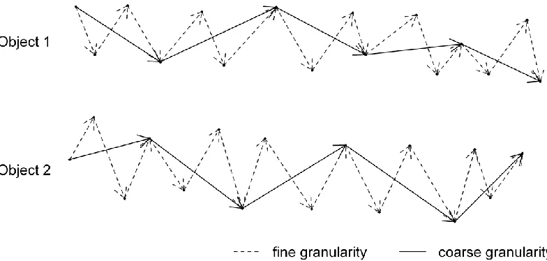
342

shows that a substantial level of interaction exists between the two athletes (DI = 0.572). 343

Local analysis enables the identification of times/locations where the athletes exhibit 344

more or less interactive movements (Figure 5). In the ultimate frisbee example, local 345

analysis is more informative than the global measure, as the movement path consists of 346

many (shorter) movement segments. Maps of local di can be combined with a time-series 347

graph of di, diθ, and did related to times/locations during the game where the defending 348

player did a poor job covering the offensive player. We use episodal level analysis to 349

segregate the movement paths into episodes of high vs. low interaction in order to further 350

- 40 seconds (highlighted in blue in Figure 5), high and positive di values suggest the 352

defending player is providing good defensive coverage (for these two episodes DI = 353

0.757). While from 20 - 38 seconds (highlighted in red in Figure 5) di values are much 354

lower, an indication of less interactive movement and poor defensive coverage (for this 355

episode DI = 0.122). 356

< Approximate location of Figure 5 > 357

5.3 Grizzly Bears in Alberta, Canada 358

In the grizzly bear example it was revealed that the male and female bears showed 359

substantial interaction (DI = 0.578) over the 42 day period from May 28, 2000 to July 8, 360

2000, using time-based weighting (see equation (11)) to account for missing fixes. 361

Similarly, time weighted results for azimuth (DIθ = 0.663) and displacement (DId = 362

0.731) reveal that both azimuth and displacement were strongly related during this 363

period. Local analysis revealed that the strong interaction seen with the global results was 364

a function of highly cohesive movements during the middle of June, while at the 365

beginning of June the two animals show little interaction (see Figure 6). Again we 366

perform analysis at the episodal level for separate periods identified visually from the 367

local analysis as having low and high dynamic interaction (low interaction: May 28 – 368

June 09; high interaction: June 09 – 29). The period of high interactions has a time-369

weighted DI = 0.492, while the period of low interaction has a time-weighted DI = 0.029. 370

Highly interactive behavior by mating grizzly bears is common in this region, as males 371

will attempt to confine female movements to a ‘mating area’ (Hamer and Herrero 1990). 372

Interpretation of maps and graphs of di facilitates the identification of where and when 373

< Approximate location of Figure 6 > 375

6 Discussion

376

DI has three fundamental advantages over an existing method (Shirabe 2006) for 377

measuring interactions (termed correlations) in movement data. First, the existing method 378

follows a traditional correlation coefficient structure and is thus dependent on the mean 379

vector of a movement vector time series. In most cases, this mean movement vector will 380

have little relevance in the context of the analysis. However, in cases where interactions 381

are expected to occur relative to some mean movement trajectory, the method from 382

Shirabe (2006) is still advantageous. For instance, two objects moving radially from a 383

point (at some acute angle) may exhibit dynamic interaction (e.g., Fig. 4a in Shirabe 384

2006). Second, DI is explicitly decomposed into components measuring interaction in 385

movement azimuth and displacement. This property enables analysts to identify 386

situations where movements are related in one component but not the other. For example, 387

in scenario 3, DId is low, however strong interaction is present in DIθ, indicating that the

388

objects move with similar azimuths but not displacements, a conclusion not discernable 389

from the rxy statistic. Lastly, the di statistics we have developed are calculated

390

independently for each simultaneous movement segment. The di values can be mapped 391

and analyzed in a time-series fashion providing a local level analysis. Local analysis 392

reveals spatial-temporal information about locations of increased or decreased interaction 393

along the movement trajectory. Furthermore, the local level statistics (di, diθ, and did) are 394

easily aggregated to coarser levels of analysis (interval, episodal, and global). 395

Other research areas where measuring movement interactions could provide new 396

examples. In transportation applications measuring interactions in large movement 398

databases could be used for generating information on commuter behavior. Examples 399

from human-activity research where interactions are important include tourist behavior 400

(e.g., Shoval and Isaacson 2007) or crowd dynamics (Batty et al. 2003). With wildlife 401

movement data, the detection of interactions is important in the study of resource 402

selection (Millspaugh et al. 1998) and social behavior (Bandeira de Melo et al. 2007; 403

Kenward et al. 1993), but also for examining offspring dependency, and inter-/intra-404

species behavior. Finally, a number of sporting examples exist where measuring 405

movement interactions could provide new and unique insight including soccer, American 406

football, and ice hockey. 407

We use simulated movement data to highlight the advantages of DI over an 408

existing method in a small set of specific scenarios designed to show the range of 409

dynamic interactions present in movement data. When two movements are highly 410

interactive (e.g., scenario 1) both methods successfully identify the high level of dynamic 411

interaction. Also, when two movements show opposing or repulsive movements (e.g., 412

scenario 4) both methods are able to identify this behavior. The value of the DI method is 413

demonstrated in scenarios 3, 4, and 5, where interactions in either azimuth or 414

displacement are coupled with no interaction in the other component. This type of 415

analysis may be useful, for example, when object movement is dependent on a temporal 416

factor. For instance, many wildlife species are active only at specific times of the day and 417

remain dormant during other periods. Measuring positive dynamic interactions in 418

different species or individuals operate with similar circadian cycles (Merrill and Mech 420

2003). 421

The example from athletes playing ultimate frisbee demonstrates the value of 422

measuring dynamic interactions at the local and episodal levels of analysis. Local and 423

episodal analysis revealed periods of varying degrees of dynamic interaction, which can 424

be related to player performance (i.e., how well the defensive player was able to cover the 425

offensive player). In many team sports, player evaluation has traditionally been 426

conducted by human observers. More recently, data driven analyses have become 427

common in the evaluation of players in team sports (e.g., Fearnhead and Taylor 2011). 428

When a player’s movement can be directly related to specific abilities, for instance the 429

soccer example in Laube et al. (2005), the measurement of dynamic interactions, using 430

the DI method can enhance player evaluation using novel sport-specific movement 431

datasets. 432

The DI method we have developed requires that movement locations be recorded 433

simultaneously. Such a tidy form of movement data (i.e., where objects locations are 434

recorded simultaneously) may not always be available, limiting the ability to implement 435

this method. In such cases, path interpolation methods (e.g., Tremblay et al. 2006) could 436

be used to estimate the locations of one object at coinciding times. Similarly, in many 437

applications the assumption that movement data are collected at a regular interval is not 438

satisfied (e.g., with movement data collected using cell-phone records). This is also the 439

case in many wildlife telemetry studies where missing fixes are common. In the grizzly 440

bear example, we demonstrate the value of temporal weighting the DI statistic to account 441

can provide unique and valuable insights into the nature of dynamic interactions present 443

in movement datasets. Local analysis reveals the times and locations of dynamic 444

interactions not discernable from global level statistics. When comparing male and 445

female grizzly bears, the dynamic interactions were likely due to mating behavior. This 446

example demonstrates the value of quantifying dynamic interactions in wildlife 447

movement datasets, as they can be related directly to specific social activities. 448

When movement data are collected at too fine a granularity, the movement 449

process (e.g., dynamic interaction) can be masked by data noise (termed over-sampling, 450

Turchin 1998). In these cases, down-sampling can be used to reduce data redundancy in 451

the movement path and improve the process signal to noise ratio. The DI statistics can 452

then be computed on the re-sampled movement dataset, as another form of interval and/or 453

episodal analysis (e.g., Laube et al. 2007). Variations of this procedure at different 454

interval and episodal scales can lead to increasingly complex and cross-scale 455

investigations of dynamic interactions in moving object datasets. Recently, Laube and 456

Purves (2011) have discussed the impact that movement data granularity (i.e., sampling 457

resolution) has on metrics used to quantify and describe movement trajectories (e.g., 458

mean speed). The DI method is similarly impacted by the granularity at which 459

movement data are represented. For example, at a coarse granularity objects may exhibit 460

positive dynamic interactions, while at a fine granularity their movements may show 461

negative dynamic interaction (see Figure 7). Both the granularity at which the data are 462

represented and analysis level selected will impact the results and subsequent 463

movement data analysis be conducted across a range of scales (granularities and analysis 465

levels) to correctly understand observed patterns. 466

< Approximate location of Figure 7 > 467

6 Conclusions

468

Movement data are being collected for a variety of research agendas involving the 469

study of humans, their vehicles, and wildlife. Central to analyzing movement data is the 470

measurement of dynamic interactions between pairs of moving objects. We have 471

developed a new statistic (DI) for measuring dynamic interactions in discrete movement 472

data (e.g., with a GPS). The basic properties of movement segments – azimuth and 473

displacement, are used to detect dynamic interactions in azimuth, displacement, and 474

overall movement. The DI method can be applied at four analysis levels (local, interval, 475

episodal, and global - Laube et al. 2007) associated with movement data, and results can 476

be aggregated across analysis levels. We introduce both time- and distance-based 477

weighting schemes that can be useful in specific situations. The measurement of dynamic 478

interactions at a temporal-lag, an example of trend-setting (Laube et al. 2005), can be 479

easily incorporated. Like many spatial analysis techniques the DI method is impacted by 480

the granularity at which movement data is represented. A detailed investigation of cross-481

scale effects is warranted to provide a better understanding of how the measurement of 482

dynamic interaction is impacted by changing data granularities. 483

In some situations the nature of movement interactions will not simply involve 484

two moving objects, but rather involve two moving objects impacted by a third. Consider 485

the grizzly bear example; the bears exhibit varying levels of dynamic interaction over the 486

relative to the location of other objects, including other bears, roads, or sources of 488

attraction or repulsion (i.e., food or danger). Future research will develop approaches for 489

measuring third-party interactions, whereby pairs of moving objects interact with respect 490

to a third stationary or moving object. 491

To those wishing to measure dynamic interactions with their own applications we 492

have developed code for implementing DI in the statistical software package R (R 493

Development Core Team 2011), for more information please visit: 494

<insert link to website here> 495

Acknowledgements

496

Funding for this work was provided by Canada’s Natural Science and 497

Engineering Research Council (NSERC) and GEOIDE through the Government of 498

Canada’s Networks for Centres of Excellence program. A special thanks to G. Stenhouse 499

and the Foothills Research Institute for access to the grizzly bear data used in the case 500

study. Also, thanks go out to the University of Victoria Ultimate Frisbee Club for their 501

participation in ongoing data collection endeavors. The constructive comments we 502

received from three anonymous reviewers greatly improved the presentation of this 503

article. 504

References

506 507

Alt H and Godau M 1995 Computing the Fréchet distance between two polygonal curves. 508

International Journal of Computational Geometry & Applications 5 (1-2): 75-91 509

Bandeira de Melo L F, Lima Sabato M A, Vaz Magni E M, Young R J and Coelho C M 510

2007 Secret lives of maned wolves (Chrysocyon brachyurus Illiger 1815): as 511

revealed by GPS tracking collars. Journal of Zoology 271 27-36 512

Batty M, Desyllas J and Duxbury E 2003 The discrete dynamics of small-scale events: 513

agent-based models of mobility in carnivals and street parades. International 514

Journal of Geographical Information Science 17 (7): 673-97 515

Benkert M, Djordjevic B, Gudmundsson J and Wolle T 2007 Finding popular places. In 516

Tokuyama T (eds) Proceedings of the ISAAC 2007, LNCS 4835: 776-87 517

Benkert M, Gudmundsson J, Hubner F and Wolle T 2008 Reporting flock patterns. 518

Computational Geometry 41 111-25 519

Buchin K, Buchin M and Gudmundsson J 2010 Constrained free space diagrams: a tool 520

for trajectory analysis. International Journal of Geographical Information 521

Science 24 (7): 1101-25 522

de Lucca Siqueira F and Bogorny V 2011 Discovering chasing behavior in moving object 523

trajectories. Transactions in GIS 15 (5): 667-88 524

Doncaster C P 1990 Non-parametric estimates of interactions from radio-tracking data. 525

Journal of Theoretical Biology 143 431-43 526

Fearnhead P and Taylor B M 2011 On estimating the ability of NBA players. Journal of 527

Quantitative Analysis in Sports 7 (3): Article 11 528

Gao Y, Zheng B, Chen G and Li Q 2010 Algorithms for constrained k-nearest neighbor 529

queries over moving object trajectories. Geoinformatica 14 241-76 530

Hamer D and Herrero S 1990 Courtship and use of mating areas by grizzly bears in the 531

front ranges of Banff National Park, Alberta. Canadian Journal of Zoology 68 532

2695-97 533

Kenward R E, Marcstrom V and Karlbom M 1993 Post-nestling behaviour in goshawks, 534

Accipiter gentilis: II. Sex differences in sociality and nest-switching. Animal 535

Behaviour 46 371-78 536

Laube P, Imfeld S and Weibel R 2005 Discovering relative motion patterns in groups of 537

moving point objects. International Journal of Geographical Information Science 538

19 (6): 639-68 539

Laube P, Dennis T, Forer P and Walker M 2007 Movement beyond the snapshot - 540

Dynamic analysis of geospatial lifelines. Computers, Environment and Urban 541

Systems 31 481-501 542

Laube P and Purves R S 2011 How fast is a cow? Cross-scale analysis of movement data. 543

Transactions in GIS 15 (3): 401-18 544

Macdonald D W, Ball F G and Hough N G 1980 The evaluation of home range size and 545

configuration using radio tracking data. In Amlaner C J and Macdonald D W 546

(eds) A Handbook on Biotelemetry and Radio Tracking. Oxford, Pergamon Press: 547

405-24 548

Merrill S B and Mech L D 2003 The usefulness of GPS telemetry to study wolf circadian 549

Millspaugh J J, Skalski J R, Kernohan B J, Raedeke K J, Brundige G C and Cooper A B 551

1998 Some comments on spatial independence in studies of resource selection. 552

Wildlife Society Bulletin 26 (2): 232-36 553

Noyon V, Claramunt C and Devogele T 2007 A relative representation of trajectories in 554

geographical spaces. Geoinformatica 11 479-96 555

R Development Core Team 2011 R: A language and environment for statistical 556

computing. R Foundation for Statistical Computing. ISBN 3-900051-07-0, URL 557

http://www.R-project.org Vienna, Austria

558

Shirabe T 2006 Correlation analysis of discrete motions. In Raubal M, Miller H J, Frank 559

A U and Goodchild M F (eds) GIScience 2006. LNCS, vol. 4197. Berlin, 560

Springer-Verlag: 370-82 561

Shoval N and Isaacson M 2007 Sequence alignment as a method for human activity 562

analysis in space and time. Annals of the Association of American Geographers 563

97 (2): 282-97 564

Sinha G and Mark D M 2005 Measuring similarity between geospatial lifelines in studies 565

of environmental health. Journal of Geographical Systems 7 115-36 566

Stenhouse G B, Boulanger J, Lee J, Graham K, Duval J and Cranston J 2005 Grizzly bear 567

associations along the eastern slopes of Alberta. Ursus 16 (1): 31-40 568

Tremblay Y, Shaffer S A, Fowler S L, Kuhn C E, McDonald B I, Weise M J, Bost C A, 569

Weimerskirch H, Crocker D E, Goebel M E and Costa D P 2006 Interpolation of 570

animal tracking data in a fluid environment. The Journal of Experimental Biology 571

209 128-40 572

Turchin P 1998 Quantitative Analysis of Movement: Measuring and Modelling 573

Population Redistribution in Animals and Plants. Sunderland, MA, Sinauer 574

Vlachos M, Gunopulos D and Kollios G 2002 Robust similarity measures for mobile 575

object trajectories. In (eds) Proceedings of the 5th International Workshop on 576

Mobility in Databases and Distributed Systems (MDDS), Aix-en-Provence, 577

France: 721-26 578

Wolfer D P, Madani R, Valenti P and Lipp H-P 2001 Extended analysis of path data from 579

mutant mice using the public domain software Wintrack. Physiology & Behavior 580

73 745-53 581

Yanagisawa Y, Akahani J I and Satoh T 2003 Shape-based similarity query for trajectory 582

of mobile objects. In Chen M-S, Chysanthis P K, Sloman M and Zaslavsky A 583

(eds) Mobile Data Management, LNCS 2574. Berlin, Springer-Verlag: 63-77 584

Table 1: Simulated movement scenarios, depicting different types of dynamic

interactions, used to examine the differences between the new interaction statistic (DI) and an existing method (r).

Scenario Azimuth (θ) Displacement (d) 1 Positive interaction Interaction

2 Positive interaction (rotated by 45°)

Interaction

3 Positive interaction No interaction

4 Negative interaction No interaction

5 No interaction Interaction

6 Random Random

Figure 6: Local analysis showing maps of di values for a) the male grizzly bear (G006), and b) the female grizzly bear (G010), from the grizzly bear example. c) time series graphs of di, diθ, and did can be used to identify periods of high and low dynamic