Assessment of CPT based methods for liquefaction evaluation in a liquefaction potential index (LPI) framework

328

Assessment of CPT-based methods for liquefaction evaluation in a

liquefaction potential index framework

B. W. M AU R E R, R . A . G R E E N, M . C U B R I N OV S K I † a n d B. A . B R A D L E Y †

In practice, several competing liquefaction evaluation procedures (LEPs) are used to compute factors of safety against soil liquefaction, often for use within a liquefaction potential index (LPI) framework to assess liquefaction hazard. At present, the influence of the selected LEP on the accuracy of LPI hazard assessment is unknown, and the need for LEP-specific calibrations of the LPI hazard scale has never been thoroughly investigated. Therefore, the aim of this study is to assess the efficacy of three CPT-based LEPs from the literature, operating within the LPI framework, for predicting the severity of liquefaction manifestation. Utilising more than 7000 liquefaction case studies from the 2010–2011 Canterbury (NZ) earthquake sequence, this study found that: (a) the relationship between liquefaction manifestation severity and computed LPI values is LEP-specific; (b) using a calibrated, LEP-specific hazard scale, the performance of the LPI models is essentially equivalent; and (c) the existing LPI framework has inherent limitations, resulting in inconsistent severity predictions against field observa-tions for certain soil profiles, regardless of which LEP is used. It is unlikely that revisions of the LEPs will completely resolve these erroneous assessments. Rather, a revised index which more adequately accounts for the mechanics of liquefaction manifestation is needed.

KEYWORDS: earthquakes; liquefaction; sands; seismicity

INTRODUCTION

The objective of this study is to assess the efficacy of three common cone penetration test (CPT)-based liquefaction eva-luation procedures (LEPs), operating within a liquefaction potential index (LPI) framework, for predicting the severity of surficial liquefaction manifestation, which is commonly used as a proxy for liquefaction damage potential. Utilising data from the 2010–2011 Canterbury earthquakes, this study investigates the influence of the selected LEP on the accu-racy of hazard assessments, and assesses the need for LEP-specific calibrations of the LPI hazard scale. Towards this end, the deterministic LEPs of Robertson & Wride (1998) (R&W98), Moss et al. (2006) (MEA06), and Idriss & Boulanger (2008) (I&B08) are evaluated.

While the ‘simplified’ LEP (Seed & Idriss, 1971; Whit-man, 1971) is central to most liquefaction hazard assess-ments, the output from an LEP is not a direct quantification of liquefaction damage potential, but rather is the factor of safety against liquefaction triggering (FSliq) in a soil stratum at depth. Iwasaki et al. (1978) proposed the LPI to link liquefaction triggering at depth to damage potential, where LPI is computed as

LPI¼ ð

20 m

0

Fw(z)dz (1)

where F¼1FSliq for FSliq<1 and F¼0 for FSliq.1; w(z) is a depth weighting function given byw(z)¼100.5z; andzis depth in metres below the ground surface. Thus, it is

assumed that the severity of liquefaction manifestation is proportional to the thickness of a liquefied layer, the proxi-mity of the layer to the ground surface, and the amount by which FSliq is less than 1.0. Given this definition, LPI can range from 0 to a maximum of 100 (i.e. where FSliq is zero over the entire 20 m depth). Analysing SPT data from 55 sites in Japan, Iwasaki et al. (1978) proposed that severe liquefaction should be expected for sites where LPI.15 but not where LPI,5. This criterion for liquefaction manifesta-tion, defined by two threshold values of LPI, is subsequently referred to as the Iwasaki criterion. However, in using the LPI framework to assess liquefaction hazard in current prac-tice, it is not always appreciated that the Iwasaki criterion is inherently linked to the LEP that was in common use in Japan in 1978, which differs significantly from those com-monly used today. Also, it has been shown that the various LEPs used in today’s practice can result in different FSliq values for the same soil profile and earthquake scenario (e.g. Green et al., 2014), and thus different LPI values. These differences have led to confusion as to which LEP is the most accurate, and whether the Iwasaki criterion is equally effec-tive for all LEPs.

The 2010–2011 Canterbury earthquake sequence (CES) resulted in a liquefaction dataset of unprecedented size and quality, presenting a unique opportunity to assess the effi-cacy of liquefaction analytics (e.g. Cubrinovski & Green, 2010; Cubrinovski et al., 2011; Bradley & Cubrinovski, 2011). Towards this end, Maureret al. (2014) evaluated LPI during the CES at approximately 1200 sites using the R&W98 CPT-based LEP. Although the Iwasaki criterion was found to be effective in a general sense, LPI hazard assess-ments were erroneous for a portion of the study area. In practice, several competing LEPs are used to assess liquefac-tion hazard in an LPI framework (e.g. Sonmez, 2003; Toprak & Holzer, 2003; Baise et al., 2006; Holzer et al., 2006a, 2006b; Lenz & Baise, 2007; Cramer et al., 2008; Hayati & Andrus, 2008; Holzer, 2008; Chung & Rogers, 2011; Kang et al., 2014), but the need for LEP-specific calibration of the LPI hazard scale has never been thoroughly investigated.

Manuscript received 31 March 2014; revised manuscript accepted 9 January 2015. Published online ahead of print 23 February 2015. Discussion on this paper closes on 1 October 2015, for further details see p. ii.

_{Department of Civil and Environmental Engineering, Virginia Tech,}

Blacksburg, Virginia, USA.

Therefore, the objective of this study is to assess the efficacy of the R&W98, MEA06 and I&B08 CPT-based LEPs, operating within the LPI framework, for predicting the severity of surficial liquefaction manifestation. Utilising more than 7000 liquefaction case studies from the CES, this study evaluates the influence of the selected LEP on the accuracy of hazard assessment, and assesses the need for LEP-specific calibrations of the LPI hazard scale. This evaluation is performed using receiver operating characteris-tic (ROC) analyses, which are commonly used to assess the performance of medical diagnostics (e.g. Zou, 2007).

In the following, the high-quality liquefaction case history dataset resulting from the CES is briefly summarised. This is followed by a description of how LPI was computed using three common CPT-based LEPs. An overview of ROC analyses is then presented, which is followed by the analysis of the LPI data. The influence of the LEP on the accuracy of LPI hazard assessment is then discussed.

DATA AND METHODOLOGY

The 2010–2011 CES began with the moment magnitude (Mw) 7.1, 4 September 2010 Darfield earthquake and in-cludes up to ten events that are known to have induced liquefaction in the affected region (Quigley et al., 2013). However, most notably, widespread liquefaction was induced by the Darfield earthquake and the Mw 6.2, 22 February 2011 Christchurch earthquake (e.g. Green et al., 2014). Ground motions from these events were recorded by a dense network of strong motion stations (e.g. Bradley & Cubri-novski, 2011), and due to the extent of liquefaction, the New Zealand Earthquake Commission funded an extensive geotechnical reconnaissance and characterisation programme (Murahidy et al., 2012). The combination of densely corded ground motions, well-documented liquefaction re-sponse and detailed subsurface characterisation comprises the high-quality dataset used for this study. To evaluate the influence of the LEP operating in the LPI framework, a large database of CPT soundings performed across Christchurch and its environs (CGD, 2012a) are analysed in conjunction with liquefaction observations made following the Darfield and Christchurch events.

CPT soundings

This study utilises 3616 CPT soundings performed at sites where the severity of liquefaction manifestation was well documented following both the Darfield and Christchurch earthquakes, resulting in more than 7000 liquefaction case studies. In the process of compiling these case studies, CPT soundings were first rejected from the study as follows. First, CPTs were rejected if the depth of ‘pre-drill’ significantly exceeded the estimated depth of the ground-water table (GWT), a condition arising at sites where buried utilities needed to be safely bypassed before testing could begin. Second, to identify soundings prematurely terminating on shallow gravels, termination depths of CPT soundings were geo-spatially analysed using an Anselin local Moran’s I analysis (Anselin, 1995) and soundings with anomalously shallow termination depths were removed from the study. For a complete discussion of CPT soundings and the geospa-tial analysis used herein, see Maureret al.(2014).

Liquefaction severity

Observations of liquefaction and the severity of manifesta-tions were made by the authors for each of the CPT sounding locations following both the Darfield and Christch-urch earthquakes. This was accomplished by ground

recon-naissance and using high-resolution aerial and satellite imagery (CGD, 2012b) performed in the days immediately following each of the earthquakes. CPT sites were assigned one of six damage classifications, as described in Table 1, where the classifications describe the predominant damage mechanism and manifestation of liquefaction. For example, some ‘severe liquefaction’ sites also had minor lateral spreading, and likewise, many ‘lateral spreading’ sites also had some amount of liquefaction ejecta present. Of the more than 7000 cases compiled, 48% are cases of ‘no manifesta-tion’, and 52% are cases where manifestations were ob-served and classified in accordance with Table 1.

Estimation of amax(peak ground acceleration)

To evaluate FSliq using the three LEPs (i.e. R&W98, MEA06 and I&B08), the peak ground accelerations (PGAs) at the ground surface were computed using the robust procedure discussed in detail by Bradley (2013a) and used by Green et al. (2011, 2014) and Maureret al. (2014). The Bradley (2013a) procedure combines unconditional PGA distributions estimated by the Bradley (2013b) ground motion prediction equation, recorded PGAs from strong motion stations, and the spatial correlation of intra-event residuals to compute the conditional PGA distribution at sites of interest.

Estimation of ground-water table depth

Given the sensitivity of liquefaction hazard and computed LPI values to GWT depth (e.g. Chung & Rogers, 2011; Maurer et al., 2014), accurate measurement of GWT depth is critical. For this study, GWT depths were sourced from the robust, event-specific regional ground-water models of van Ballegooy et al. (2014). These models, which reflect seasonal and localised fluctuations across the region, were derived in part using monitoring data from a network of

,1000 piezometers and provide a best estimate of GWT depths immediately prior to the Darfield and Christchurch earthquakes.

Liquefaction evaluation and LPI

The value of FSliq was computed using the deterministic CPT-based LEPs of R&W98, MEA06 and I&B08, where the soil behaviour type index, Ic, was used to identify

Table 1. Liquefaction severity classification criteria (after Green

et al., 2014)

Classification Criteria

No manifestation No surficial liquefaction manifestation or lateral spread cracking

Marginal manifestation

Small, isolated liquefaction features; streets had traces of ejecta or wet patches less than a vehicle width;,5% of ground surface covered by ejecta Moderate

manifestation

Groups of liquefaction features; streets had ejecta patches greater than a vehicle width but were still passable; 5–40% of ground surface covered by ejecta

Severe manifestation

Large masses of adjoining liquefaction features, streets impassable owing to liquefaction;.40% of ground surface covered by ejecta

Lateral spreading Lateral spread cracks were predominant manifestation and damage mechanism, but crack displacements,200 mm

Severe lateral spreading

Extensive lateral spreading and/or large open cracks extending across the ground surface with

non-liquefiable strata; soils having Ic.2.6 were considered too plastic to liquefy. Soil unit weights were estimated for each procedure using the method of Robertson & Cabal (2010). For the MEA06 procedure, the stress-reduction coef-ficient, rd, was computed using the Vs-independent equation given in Moss et al. (2006); in addition, the probability of liquefaction (PL) was set to 0.15, as proposed by Mosset al. (2006) for deterministic assessments of FSliq. For the I&B08 procedure, fines content (FC) is required to compute normal-ised tip resistances (in lieu of FC, R&W98 and MEA06 use Ic and CPT friction ratio, Rf, respectively); as such, FC values were estimated using both the genericIc–FC correla-tion proposed by Robertson & Wride (1998) and a Christch-urch-soil-specific Ic–FC correlation developed by Robinson et al. (2013). Henceforth herein, I&B081 _{and I&B08}2 _refer to the use of the generic and Christchurch-specific Ic–FC correlations, used in conjunction with the I&B08 procedure. The two Ic–FC correlations are shown in Fig. 1; it can be seen that the Christchurch-specific correlation suggests dif-ferent Ic–FC trends for Ic,1.7 and Ic>1.7, where FC is estimated to be 10 for all Ic<1.7. While thin layer correc-tions (i.e. adjustments to CPT data in thin strata to account for the influence of over- or underlying soils) are applicable to the LEPs used herein, their use requires judgement, and an automated implementation of these corrections does not yet exist. Given the quantity of case studies analysed, thin layer corrections were not performed. FSliqwas computed at 1- or 2-cm depth intervals (i.e. the measuring rate of CPT soundings); LPI was then computed with each of the four LEPs as per equation (1).

OVERVIEW OF ROC ANALYSES

Receiver operating characteristic analyses are used herein to assess: (a) the efficacy of each LEP for predicting the severity of liquefaction manifestation within the LPI frame-work; and (b) the need for LEP-specific calibrations of the LPI hazard scale. ROC analyses have been extensively used in assessing medical diagnostic tests in clinical studies (e.g. imaging tests for identifying abnormalities), as well as in machine learning and data-mining research (e.g. Swets et al., 2000; Eng, 2005; Fawcett, 2006; Metz, 2006). In any ROC application, the distributions of ‘positives’ (e.g. lique-faction is observed) and ‘negatives’ (e.g. no liquelique-faction is observed) overlap when the frequency of the distributions are expressed as a function of index test results (e.g. LPI values). In such cases, threshold values for the index test results are selected considering the relative probabilities of

true positives (i.e. liquefaction is observed, as predicted) and false positives (i.e. liquefaction is predicted, but is not observed). Setting the threshold too low will result in numerous false positives, which is not without consequences, while setting the threshold unduly high will result in many false negatives (i.e. liquefaction is observed when it is predicted not to occur), which comes with a different set of consequences. ROC analyses are particularly valuable for evaluating the relative efficacy of competing diagnostic tests, independent of the thresholds used, and for selecting an optimal threshold for a given diagnostic test.

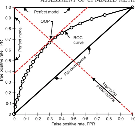
In this study, the competing diagnostic tests are the LEPs, and the index test results are the computed LPI values. Accordingly, in analysing the case histories, true and false positives are scenarios where surficial liquefaction manifesta-tions are predicted, but were and were not observed, respec-tively. Fig. 2 illustrates the relationship among the positive and negative distributions, the selected threshold value and the corresponding ROC curve, where the ROC curve plots the true positive rate (TPR) and false positive rate (FPR) for varying threshold values. Fig. 3 illustrates how a ROC curve is used to assess the efficiency of LPI hazard assessment,

0 10 20 30 40 50 60 70 80 90 100

1·25 1·50 1·75 2·00 2·25 2·50 2·75 3·00 3·25 3·50

A

pparent fines content, FC: %

Soil behaviour type index,Ic Christchurch-specific correlation (REA13)

Generic correlation (R&W98)

R&W98

high-plasticity bound R&W98

low-plasticity bound

Fig. 1. Correlations betweenIcand apparent FC: Christchurch-specific correlation (Robinsonet al., 2013) and generic correlation (Robertson & Wride, 1998)

0 0·1 0·2 0·3 0·4 0·5 0·6 0·7 0·8 0·9 1·0

0 0·1 0·2 0·3 0·4 0·5 0·6 0·7 0·8 0·9 1·0

T

rue positi

v

e

r

a

te

, TPR

False positive rate, FPR (b)

B LPI⫽8·75

A LPI⫽5

C LPI⫽14

D LPI⫽18

ROC curve

Increasing LPI threshold

0 2·5 5·0 7·5 10·0 12·5 15·0 17·5 20·0 22·5

F

requency

Liquefaction potential index, LPI (a)

No surficial liquefaction manifestation

Surficial liquefaction manifestation

A LPI⫽5

B 8·75

C 14

D 18

where TPR and FPR are synonymous with ‘true positive probability’ and ‘false positive probability’, respectively. In ROC curve space, random guessing is indicated by a 1:1 line through the origin (i.e. equivalent correct and incorrect pre-dictions), while a perfect model plots as a point at (0,1), indicating the existence of a threshold value which perfectly segregates the dataset (e.g. all sites with manifestation have LPI above the selected threshold; all sites without manifesta-tion have LPI below the same selected threshold). While no single parameter can fully characterise model performance, the area under a ROC curve (AUC) is commonly used for this purpose, where AUC is equivalent to the probability that sites with manifestation have higher computed LPI than sites with-out manifestation (e.g. Fawcett, 2006). As such, increasing AUC indicates better model performance. The optimum oper-ating point (OOP) is defined herein as the threshold LPI value which minimises the rate of misprediction (i.e. FPR + (1

TPR), where TPR and FPR are the rates of true and false positives, respectively). As such, contours of the quantity [FPR + (1TPR)] represent points of equivalent perform-ance in ROC space. Thus, in plotting the LPI data as ROC curves for each LEP, it is possible to assess both the influence of LEPs on the accuracy of hazard assessments, and the need for LEP-specific calibrations of the LPI hazard scale.

RESULTS AND DISCUSSION

Utilising more than 7000 combined case studies from the Darfield and Christchurch earthquakes, LPI values were computed using the LEPs of R&W98, MEA06, I&B081 _and I&B082.

Prediction of liquefaction occurrence

In Fig. 4, ROC curves are plotted to evaluate the perform-ance of each LPI model in segregating sites with and with-out liquefaction manifestation; this initial analysis assesses only whether LPI accurately predicts the occurrence of manifestations and does not yet consider manifestation se-verity. Included in Fig. 4 are data from both the Darfield and Christchurch earthquakes for all investigation sites, except for those where lateral spreading was the predomi-nant manifestation (the separate assessment of lateral

spread-ing is discussed later in this paper). It can be seen in Fig. 4 that, while the four LPI models perform similarly, MEA06 and I&B081 _{are respectively the least and most efficacious,} with AUC ranging from 0.71 (MEA06) to 0.78 (I&B081). To place this performance in context, AUCs of 0.5 and 1.0, respectively, indicate random guessing and a perfect model. Also, as highlighted in Fig. 4, the optimum threshold LPI values for the R&W98, MEA06, I&B081 _{and I&B08}2 mod-els are 4.0, 5.5, 6.0 and 4.5, respectively. Thus, while the lower Iwasaki criterion (i.e. LPI¼5) is generally appropriate for predicting liquefaction manifestation in Christchurch, the optimum threshold is LEP dependent. The presence of dif-ferent optimum threshold LPI values for each LEP is not surprising given that different LEPs have been shown to commonly compute notably different FSliq values for the same soil profile (e.g. Green et al., 2014). Although not unexpected, these findings may have important implications for liquefaction hazard assessment, as the risks correspond-ing to particular LPI values depend on the LEP used to compute LPI.

Also of interest is the influence of the Ic–FC correlation used within the I&B08 LEP. As shown in Fig. 1, the Christchurch-specific correlation infers a higher FC than does the generic correlation for all values of Ic, resulting in higher computed FSliqvalues, and thus lower computed LPI. As a result, the LPI hazard scale computed using I&B082 (i.e. using the Christchurch-specific correlation) is shifted towards lower values relative to the hazard scale computed using I&B081 _{(i.e. using the generic correlation) such that} the median LPI values computed using I&B081and I&B082 are 7.2 and 4.1, respectively. In addition to influencing the LPI hazard scale, the Ic–FC correlation affects model effi-cacy (i.e. efficiency segregating sites with and without liquefaction manifestations), with I&B081 _correctly classify-ing 3% more cases than I&B082 _{when operating at their} respective OOPs. The slightly weaker performance of I&B082 _{might be due to the fact that the Robinson et al.} (2013) Christchurch-specific Ic–FC correlation was devel-oped using data from along the Avon River only, while the database assessed herein consists of sites distributed through-out Christchurch, although further analysis is needed to evaluate this hypothesis. As research continues in Christ-church, refined region-specific Ic–FC correlations, which Impro

ving perf

or mance Random

guess

0 0·1 0·2 0·3 0·4 0·5 0·6 0·7 0·8 0·9 1·0

0 0·1 0·2 0·3 0·4 0·5 0·6 0·7 0·8 0·9 1·0

T

rue positi

v

e

r

a

te

, TPR

False positive rate, FPR

P

erf

ect model

Perfect model

ROC curve OOP

Fig. 3. Illustration of how a ROC curve is used to assess the efficiency of a diagnostic test. The optimum operating point (OOP) indicates the threshold value for which the misprediction rate is minimised, as described in the text

Iso-perf ormance

line

0·60 0·65 0·70 0·75 0·80

0·20 0·25 0·30 0·35 0·40 4·0 6·0

5·5 4·5

0 0·1 0·2 0·3 0·4 0·5 0·6 0·7 0·8 0·9 1·0

0 0·1 0·2 0·3 0·4 0·5 0·6 0·7 0·8 0·9 1·0

T

rue positi

v

e

r

a

te

, TPR

False positive rate, FPR

R&W98 MEA06 I&B081 I&B082 See inset

figure

might improve the efficacy of LPI hazard assessment in Christchurch, are likely to be developed.

While the preceding ROC analysis showed that optimum threshold LPI values are LEP dependent, the implications for liquefaction hazard assessment are not intuitively clear. For example, it was shown that for the considered dataset the R&W98 and I&B081 LPI models have optimum threshold LPI values of 4.0 and 6.0, respectively, but the potential consequence of failing to account for different optimum thresholds is not easily discerned. To elucidate the signifi-cance of these differences, the probability of surficial lique-faction manifestation is computed herein using the Wilson (1927) interval for a binomial proportion. This assessment also allows for application to risk-based frameworks, com-plementing the prior evaluation of deterministic threshold values. The resulting probabilities are plotted in Fig. 5 where each data point represents one-twentieth of the corresponding dataset (,350 case histories) and is plotted as a function of the median-percentile for each data bin (i.e. 2.5th-percentile, 7.5th-percentile, and so on); also shown are third-order poly-nomial regressions for each LPI model. It can be seen from these regressions that, at an LPI value of 5.0, the probabil-ities of liquefaction manifestation corresponding to the I&B081_{, MEA06, R&W98 and I&B08}2_{LPI models are 0.44,} 0.53, 0.58 and 0.58, respectively. Conversely, using the optimum threshold LPI values found previously, the prob-abilities corresponding to the respective LPI models are 0.50, 0.55, 0.53 and 0.55. Thus, the optimum thresholds correspond to roughly the same probability of manifestation, whereas failing to account for the influence of the LEP could

result in different risk levels for the same LPI value, particularly with I&B081_.

Prediction of liquefaction severity

While prediction of the occurrence of surficial manifesta-tion is an important component of liquefacmanifesta-tion hazard analy-sis, the severity of manifestation is of greater consequence to the built environment and is thus of added importance for hazard mapping and engineering design. To investigate the capacity of each LPI model for predicting manifestation severity, additional ROC analyses were performed for each classification of severity in Table 1; the results are sum-marised in Table 2 in the form of AUC and recommended threshold LPI values. Where the prior ROC analysis assessed each model’s capacity for predicting any surficial manifesta-tion (i.e. having at least marginal severity), the additional analyses assess their ability to predict that manifestations will be of a particular severity (e.g. moderate as opposed to marginal). As mentioned previously, lateral spreading is treated separately in this study, and the ‘marginal’, ‘moder-ate’ and ‘severe’ classifications refer only to sand-blow manifestations. This distinction is made because lateral spreading is a unique manifestation associated with large permanent ground displacements, and because there are separate criteria for assessing its severity (e.g. Youd et al., 2002), including the ground slope and height of the nearest free face (e.g. river bank), among others. Consequently, although site profiles with thin liquefiable layers may have low LPI values, these sites are susceptible to lateral spread-ing if located on slopspread-ing ground or near rivers. Since the factors pertinent to lateral spreading cases are not considered in the formulation of LPI, such cases should not be used to assess its performance.

From Table 2, the following observations are made. (a) Relative trends in model performance, as suggested by

AUC, are consistent for each classification of manifesta-tion severity. While the LPI models perform similarly, the I&B081 _{and MEA06 models are consistently the most} and least efficacious, respectively.

(b) Unsurprisingly, the models are more efficient in predict-ing the incidence of liquefaction manifestation than in predicting the severity of manifestation (e.g. distinguish-ing between marginal and moderate manifestations); nonetheless, the expected severity of manifestation increases with increasing LPI.

(c) Differences in optimum threshold LPI values extend throughout the LPI hazard scale, indicating that the utility of the Iwasaki criterion varies among LEPs.

(d) Considering the potential for damage to infrastructure, lateral spreading manifestations have relatively low optimum threshold LPI values. For example, lateral

0 0·1 0·2 0·3 0·4 0·5 0·6 0·7 0·8 0·9 1·0

0 5 10 15 20

Proba

bility of

liquefaction manif

esta

tion

LPI

R&W98 MEA06 I&B081 I&B082 R&W98 (R2⫽0·99)

I&B08 (2 R2⫽0·99)

I&B08 (1 R2⫽0·99)

MEA06(R2⫽0·98)

⫾1σ

Fig. 5. Probability of liquefaction manifestation

Table 2. Summary of receiver operator characteristic (ROC) analyses

LPI Model All manifestations†

Marginal manifestation†

Moderate manifestation†

Severe manifestation†

Lateral spreading

Severe lateral spreading OOP‡ _AUC§ _OOP‡ _AUC§ _OOP‡ _AUC§ _OOP‡ _AUC§ _OOP‡ _AUC§ _OOP‡ _AUC§

R&W98 4.0 0.73 3.0 0.68 5.5 0.62 10.5 0.69 4.5 0.83 10.0 0.66 MEA06 5.5 0.71 5.0 0.66 7.5 0.60 14.0 0.68 5.0 0.83 12.0 0.64 I&B081 _{6.0 0.78 5.0 0.72 9.0 0.64 16.0 0.69 6.5 0.79 8.0 0.62}

I&B082 _{4.5 0.75 3.0 0.70 6.0 0.63 11.0 0.69 5.0 0.86 8.0 0.63}

_{Where manifestation severity is characterised as described in Table 1.}

spreading and marginal sand-blow manifestations have similar OOPs for each respective LPI model (i.e. similar LPI distributions), but the potential for damage to infrastructure is generally much greater with lateral spreading. This illustrates that while LPI may be useful for hazard assessment, the influence of local conditions on the manifestation of liquefaction must also be considered. As such, the damage potential of lateral spreading may not be well estimated by LPI.

As was done previously, the probability of manifestation is computed to assess the significance of different optimum thresholds, and to allow for application to risk-based frame-works. Because damage to infrastructure (e.g. settlement of structures, failure of lifelines and cracking of pavements) is more likely a consequence of moderate or severe liquefac-tion, these cases are used to compute the likelihood of damaging liquefaction due to sand blows, where marginal liquefaction is considered non-damaging. Using the method-ology previously discussed, the probability of moderate or severe liquefaction is plotted in Fig. 6 along with third-order polynomial regressions for each LPI model. It can be seen from these regressions that, at an LPI value of 15.0 (i.e. the upper Iwasaki criterion), the probabilities corresponding to the I&B081, MEA06, R&W98 and I&B082 LPI models are 0.37, 0.40, 0.43 and 0.47, respectively. Conversely, using the threshold LPI values found previously for severe liquefaction (Table 2), the probabilities corresponding to the respective LPI models are 0.39, 0.39, 0.38 and 0.40. Thus, the optimum thresholds correspond to roughly the same prob-ability of damaging manifestation, whereas failing to account for the influence of the LEP results in different risk levels. Similarly, the optimum thresholds for moderate liquefaction correspond to the same level of risk (,27%).

Comparative performance in an applied framework

The preceding analyses have suggested the four LPI models may be capable of assessing liquefaction hazard, but that LEP-specific correlations relating LPI values and sever-ity of surficial liquefaction manifestations are required. To compare LEP performance in an applied setting, and to determine whether any LEP is superior for practical intents and purposes, deterministic ‘prediction errors’ are computed for each case history using both the Iwasaki criterion and

the LEP-specific calibrations in Table 2. The prediction error (E) is computed using the thresholds assigned to each manifestation category, such thatE¼LPI(min or max) of the relevant range. For example, using the Iwasaki criterion, if the computed LPI is 14 for a site with no manifestation, E¼145¼9 (where 5 is the maximum of the range of LPI values for no manifestation), whereas if the computed LPI is 6 for a site with severe liquefaction, E¼615¼ 9 (where 15 is the minimum of the range of LPI values for severe liquefaction). Thus, positive errors indicate over-predictions of manifestation severity and, conversely, nega-tive errors indicate under-predictions. While there is no precedent for using a ‘moderate manifestation’ threshold with the Iwasaki criterion, an LPI value of 8.0 is used herein to facilitate comparisons among the models. Also, in light of the separate criteria for assessing lateral spreads, lateral spreading is assigned a wide range of expected LPI values consistent with any manifestation, independent of spreading severity (i.e. lateral spread sites are only expected to have LPI>the threshold for marginal liquefaction).

The distributions of LPI prediction errors are shown for each model in Fig. 7 using both the Iwasaki (Fig. 7(a)) and LEP-specific (Fig. 7(b)) hazard scales. It can be seen in Fig. 7(a) that the distributions of errors among LEPs vary using the Iwasaki criterion, as expected. Because the models have different LPI hazard scales, applying the Iwasaki criterion to each results in dissimilar performance. For example, R&W98 and I&B081_{under-predict manifestation severity for} 38% and 18% of cases, respectively. Conversely, using the

0 0·1 0·2 0·3 0·4 0·5 0·6

0 5 10 15 20

Proba

bility of

moder

a

te or se

v

ere manif

esta

tion

LPI R&W98

MEA06 I&B081 I&B082

R&W98 (R2⫽0·98) I&B08 (2 _R2_⫽0·99)

I&B08 (1 R2⫽0·98) MEA06 (R2⫽0·97)

⫾1σ

Fig. 6. Probability of moderate or severe liquefaction manifesta-tion

0 5 10 15 20 25 30 35 40 45 50

⫺25 ⫺20 ⫺15 ⫺10 ⫺5 0 5 10 15 20 25

Prediction r

a

te (7232 cases): %

Prediction error: LPI units (a)

R&W98

MEA06

I&B081

I&B082

35% 40% 45%

⫺0·2 0 0·2

0 5 10 15 20 25 30 35 40 45 50

⫺25 ⫺20 ⫺15 ⫺10 ⫺5 0 5 10 15 20 25

Prediction r

a

te (7232 cases): %

Prediction error: LPI units (b)

R&W98

MEA06

I&B081

I&B082

35% 40% 45%

⫺0·2 0 0·2

LEP-specific calibrations of the LPI hazard scale (Fig. 7(b)), the distributions of errors among LEPs are more similar. For example, R&W98 and I&B081 _{under-predict manifestation} severity for 24% and 20% of cases, respectively. In addition, the rate of accurate prediction (i.e. zero error) is improved for each LEP; R&W98, MEA06, I&B081 _{and I&B08}2 accurately predict 44%, 42%, 46% and 44% of cases, re-spectively. These performance trends mirror those of the ROC analyses, which indicated that, although the models performed similarly, I&B081 _{and MEA06 were respectively} the most and least efficacious. However, although accurate predictions of manifestation severity are important, so too is limiting the rate of highly erroneous predictions, which are not necessarily mutually inclusive. While I&B081 has the most zero-error predictions (46%), it also has the most predictions with |E|.15 (5%). Conversely, MEA06 has the least zero-error predictions (42%), but it also has the fewest predictions with |E|.15 (2.5%). Given these inconsisten-cies, and considering the variety of metrics that might be used to gauge performance, it is difficult to argue that any one LEP is superior in this applied framework. Thus, using the LEP-specific hazard scales, and based on the prediction errors computed herein, the performance of the LPI models is, for practical intents and purposes, equivalent.

While minor errors are to be expected in any deterministic analysis, each model produced significant errors with con-sequences for hazard assessment. For example, even with calibration, |E| exceeded 10 at 9% of sites, on average, for each model (e.g. severe manifestation predicted, but no manifestation observed) and |E| exceeded 5 at 22% of sites, on average, for each model (e.g. no manifestation predicted, but moderate manifestation observed). To determine whether certain models perform better in particular locations, predic-tion errors from the calibrated R&W98, MEA06 and I&B082 _{models are plotted against one another in Fig. 8. It} can be seen that prediction errors are generally equivalent; in all, the difference in prediction error between any two of the models exceeds 5 for only 12% of investigation sites. Thus, locations of under-, over- and accurate prediction are generally consistent between models. In addition, maps showing the spatial distributions of errors to be very similar in both earthquakes are provided in an electronic supplement to this paper. Thus, some site profiles have very poor predictions, irrespective of the LEP used (note that Maurer et al. (2014) found no correlation between prediction errors and either PGA uncertainty, ground water fluctuation or CPT termination depth). This suggests that LPI has inherent limitations in its formulation, such that the variables influ-encing surficial manifestation are not adequately accounted for. While liquefaction triggering has garnered significant research and is a subject of frequent debate, the mechanics of liquefaction manifestation have received less attention. This study highlights that triggering and manifestation are two distinct phenomena contributing to liquefaction hazard, and that an improved framework providing clear separation and accounting of the two phenomena is needed.

Lastly, the 12% of cases with inconsistent prediction errors between models can be shown to correspond to ‘exceptional’ site profiles. Since the LEP-specific calibrations are based on the entire dataset (i.e. predominant behaviour across Christchurch), predictions for site profiles that diverge from typical conditions may be inconsistent among models. As an example, it can be seen in Figs 8(a) and 8(c) that a number of cases exist where the MEA06 prediction error significantly differs from that of R&W98 and I&B082_{. One} common cause of this discrepancy is cases where relatively thick, potentially liquefiable layers are present at depths greater than ,10 m. For such cases the LEPs can yield divergent FSliqand hence divergent LPI values. However, the

LEP-specific calibrations do not account for this divergence because the median cumulative thickness of soil strata predicted to liquefy below 10 m depth for all the sites in the dataset is only 0.35 m, according to I&B082_{. This} empha-sises that assessments and/or calibrations of the LPI hazard scale are a function not only of the selected LEP, but also of the chosen dataset, including the geometry and soil charac-teristics of site profiles, as well as the amplitude and dura-tion of ground shaking. As such, the applicability of findings derived herein to other datasets is unknown.

⫺15

⫺5 5 15 25 35

MEA06 prediction er

ror

: LPI units

Christchurch

Darfield | |E ⫽5

⫺15 ⫺5 5 15 25 35 MEA06 prediction error: LPI units

(a)

⫺15

⫺5 5 15 25 35

I&B08

prediction er

ror

: LPI units

2

Christchurch

Darfield

⫺15 ⫺5 5 15 25 35 MEA06 prediction error: LPI units

(b)

⫺15

⫺5 5 15 25 35

⫺15 ⫺5 5 15 25 35

I&B08

prediction er

ror

: LPI units

2

MEA06 prediction error: LPI units (c)

Christchurch

Darfield

SUMMARY AND CONCLUSIONS

Utilising high-quality case histories from the CES, this study evaluated the performance of the R&W98, MEA06, I&B081 and I&B082 CPT-based LEPs, operating within the LPI framework, for assessing liquefaction hazard. The find-ings are summarised as follows.

(a) For deterministic analyses, the optimum threshold LPI values for assessing liquefaction hazard were unique to the LEP used in the LPI framework; suggested optimum thresholds for the CES dataset are summarised in Table 2. The use of LPI for assessing lateral spread potential is not recommended.

(b) Taking these LEP-specific threshold values into account, receiver-operating-characteristic analyses indicated that, while the models performed similarly, the I&B081 _and MEA06 models were respectively the most and least efficacious.

(c) LPI probability curves were computed to assess the significance of different optimum thresholds, and to allow for application in probabilistic frameworks. The optimum thresholds were shown to correspond to roughly the same probability of manifestation, whereas failing to account for the influence of the LEP (i.e. using the Iwasaki criterion) resulted in different risk levels for the same LPI value.

(d) To compare model performance in a practical setting, deterministic ‘prediction errors’ were computed for each case history. Using the Iwasaki criterion, the distributions of errors among LEPs varied. These distributions became more similar using the LEP-specific hazard scales given in Table 2, which also improved the rate of accurate prediction for all LEPs.

(e) Even with calibration, each model had significant prediction errors (e.g. severe manifestation predicted, but no manifestation observed). This suggests that LPI has inherent limitations in its formulation, such that the variables influencing surficial liquefaction manifestation are not adequately accounted for.

(f) The findings presented in this study are based on a dataset from the CES; the applicability of these findings to other datasets is unknown.

In conclusion, the following points can be made.

(a) The risk levels corresponding to the Iwasaki criterion varied among LEPs.

(b) Using a calibrated, LEP-specific hazard scale, the performance of the LPI models was, for practical intents and purposes, equivalent.

(c) The existing LPI framework has inherent limitations such that all LEPs have very poor predictions for certain soil profiles. It is unlikely that revisions of the LEPs will completely resolve these erroneous assessments. Rather, a revised index which more adequately accounts for the mechanics of liquefaction manifestation is needed.

ACKNOWLEDGEMENTS

This study is based on work supported by the US National Science Foundation (NSF) grants CMMI 1030564, CMMI 1407428 and CMMI 1435494 and US Army Engineer Research and Development Center (ERDC) grant W912HZ-13-C-0035. The third and fourth authors would like to acknowledge the continuous financial support provided by the Earthquake Commission (EQC) and Natural Hazards Research Platform (NHRP), New Zealand, for the research and investigations related to the 2010–2011 Canterbury earthquakes. The authors also acknowledge the New Zealand GeoNet project and its sponsors EQC, GNS Science and

Land Information New Zealand (LINZ) for providing the earthquake occurrence data and the Canterbury Geotechnical Database and its sponsor EQC for providing the CPT sound-ings, lateral spread observations and aerial imagery used in this study. However, any opinions, findings, and conclusions or recommendations expressed in this paper are those of the authors and do not necessarily reflect the views of NSF, ERDC, EQC, NHRP or LINZ.

SUPPLEMENTAL DATA

The following are available in an electronic supplement: (a) aerial images representative of the liquefaction manifes-tation severity classes described in Table 1; and (b) map figures showing the spatial distribution of LPI prediction errors for each LPI model, for both the Darfield and Christchurch earthquakes.

NOTE

Some of the data used in this study were extracted from the Canterbury Geotechnical Database (https://canterbury geotechnicaldatabase.projectorbit.com), which was prepared and/or compiled for the Earthquake Commission (EQC) to assist in assessing insurance claims made under the Earth-quake Commission Act 1993 and/or for the Canterbury Geotechnical Database on behalf of the Canterbury Earth-quake Recovery Authority (CERA). The source maps and data were not intended for any other purpose. EQC, CERA and their data suppliers, and their engineers, Tonkin & Taylor, have no liability for any use of these maps and data or for the consequences of any person relying on them in any way.

NOTATION

Ic soil behaviour type index PL probability of liquefaction

Rf cone penetration test friction ratio rd stress reduction coefficient Vs shear wave velocity

w(z) depth weighting function given by w(z)¼100.5z z depth below ground surface (m)

ó standard deviation

REFERENCES

Anselin, L. (1995). Local indicators of spatial association – LISA.

Geographical Anal.27, No. 2, 93–115.

Baise, L. G., Higgins, R. B. & Brankman, C. M. (2006). Liquefac-tion hazard mapping-statistical and spatial characterizaLiquefac-tion of susceptible units. J. Geotech. Geoenviron. Engng 132, No. 6, 705–715.

Bradley, B. A. & Cubrinovski, M. (2011). Near-source strong ground motions observed in the 22 February 2011 Christchurch earthquake.Seismol. Res. Lett.82, No. 6, 853–865.

Bradley, B. A. (2013a). Estimation of site-specific and spatially-distributed ground motion in the Christchurch earthquakes: Ap-plication to liquefaction evaluation and ground motion selection for post-event investigation. Proceedings of the 19th New Zeal-and geotechnical symposium, Queenstown, New Zealand, p. 8. Bradley, B. A. (2013b). A New Zealand-specific pseudo-spectral

acceleration ground-motion prediction equation for active shal-low crustal earthquakes based on foreign models. Bull. Seismol. Soc. Am.103, No. 3, 1801–1822.

CGD (Canterbury Geotechnical Database) (2012a). Geotechnical investigation data. Map layer CGD0010. See https://canterbury geotechnicaldatabase.projectorbit.com (accessed 12/01/2012). CGD (2012b). Aerial photography. Map layer CGD0010. See

https://canterburygeotechnicaldatabase.projectorbit.com (accessed 12/01/2012).

evaluation of liquefaction potential in the St. Louis Area.

J. Geotech. Geoenviron. Engng137, No. 5, 505–515.

Cramer, C. H., Rix, G. J. & Tucker, K. (2008). Probabilistic liquefaction hazard maps for Memphis, Tennessee.Seismol. Res. Lett.79, No. 3, 416–423.

Cubrinovski, M. & Green, R. A. (2010). Geotechnical reconnais-sance of the 2010 Darfield (Canterbury) earthquake. Bull. New Zealand Soc. Earthquake Engng43, No. 4, 243–320.

Cubrinovski, M., Bradley, B., Wotherspoon, L., Green, R., Bray, J., Woods, C., Pender, M., Allen, J., Bradshaw, A., Rix, G., Taylor, M., Robinson, K., Henderson, D., Giorgini, S., Ma, K., Winkley, A., Zupan, J., O’Rourke, T., DePascale, G. & Wells, D. (2011). Geo-technical aspects of the 22 February 2011 Christchurch earthquake.

Bull. New Zealand Soc. Earthquake Engng43, No. 4, 205–226. Eng, J. (2005). Receiver operating characteristic analysis.Academic

Radiol.12, No. 12, 909–916.

Fawcett, T. (2006). An introduction to ROC analysis. Pattern Recognition Lett.27, No. 8, 861–874.

Green, R. A., Allen, A., Wotherspoon, L., Cubrinovski, M., Bradley, B., Bradshaw, A., Cox, B. & Algie, T. (2011). Performance of levees (stopbanks) during the 4 September Mw7.1 Darfield and

22 February 2011 Mw6.2 Christchurch, New Zealand,

earth-quakes.Seismol. Res. Lett.82, No. 6, 939–949.

Green, R. A., Cubrinovski, M., Cox, B., Wood, C., Wotherspoon, L., Bradley, B. & Maurer, B. (2014). Select liquefaction case histories from the 2010–2011 Canterbury earthquake sequence.

Earthquake Spectra30, No. 1, 131–153.

Hayati, H. & Andrus, R. D. (2008). Liquefaction potential map of Charleston, South Carolina based on the 1986 earthquake.

J. Geotech. Geoenviron. Engng134, No. 6, 815–828.

Holzer, T. L. (2008). Probabilistic liquefaction hazard mapping. In

Geotechnical Earthquake Engineering and Soil Dynamics IV, ASCE Geotechnical Special Publication 181 (eds D. Zeng, M. T. Manzari and D. R. Hiltunen). Reston, VA, USA: Amer-ican Society of Civil Engineers.

Holzer, T. L., Bennett, M. J., Noce, T. E., Padovani, A. C. & Tinsley, J. C. III. (2006a). Liquefaction hazard mapping with LPI in the greater Oakland, California area.Earthquake Spectra

22, No. 3, 693–708.

Holzer, T. L., Blair, J. L., Noce, T. E. & Bennett, M. J. (2006b). LIQUEMAP: A real-time post-earthquake map of liquefaction probability.Proceedings of the 8th U. S. national conference on earthquake engineering (100th anniversary earthquake confer-ence), paper no. 89. Oakland, CA, USA: Earthquake Engineer-ing Research Institute (CD-ROM).

Idriss, I. M. & Boulanger, R. W. (2008). Soil liquefaction during earthquakes, Monograph MNO-12, p. 261. Oakland, CA, USA: Earthquake Engineering Research Institute.

Iwasaki, T., Tatsuoka, F., Tokida, K. & Yasuda, S. (1978). A practical method for assessing soil liquefaction potential based on case studies at various sites in Japan.Proceedings of the 2nd international conference on microzonation for safer construction – research and application, vol. II, pp. 885–896. Arlington, VA, USA: National Science Foundation.

Kang, G. C., Chung, J. W. & Rogers, R. J. (2014). Re-calibrating the thresholds for the classification of liquefaction potential index based on the 2004 Niigata-ken Chuetsu earthquake.Engng Geol.169, 30–40.

Lenz, A. & Baise, L. G. (2007). Spatial variability of liquefaction potential in regional mapping using CPT and SPT data. Soil Dynam. Earthquake Engng27, No. 7, 690–702.

Maurer, B. W., Green, R. A., Cubrinovski, M. & Bradley, B. A. (2014). Evaluation of the liquefaction potential index for

asses-sing liquefaction hazard. J. Geotech. Geoenviron. Engng 140, No. 7, 04014032.

Metz, C. E. (2006). Receiver operating characteristic analysis: a tool for the quantitative evaluation of observer performance and imaging systems.J. Am. College Radiol.3, No. 6, 413–422. Moss, R. E. S., Seed, R. B., Kayen, R. E., Stewart, J. P., Der

Kiureghian, A. & Cetin, K. O. (2006). CPT-based probabilistic and deterministic assessment of in situ seismic soil liquefaction potential. J. Geotech. Geoenviron. Engng 132, No. 8, 1032– 1051.

Murahidy, K. M., Soutar, C. M., Phillips, R. A. & Fairclough, A. (2012). Post earthquake recovery – development of a geotechni-cal database for Christchurch central city. Proceedings of the 15th world conference on earthquake engineering, Lisbon, Por-tugal. Tokyo, Japan: International Association of Earthquake Engineering.

Papathanassiou, G. (2008). LPI-based approach for calibrating the severity of liquefaction-induced failures and for assessing the probability of liquefaction surface evidence. Engng Geol. 96, No. 1–2, 94–104.

Quigley, M., Bastin, S. & Bradley, B. (2013). Recurrent liquefaction in Christchurch, New Zealand during the Canterbury earthquake sequence.Geology41, No. 4, 419–422.

Robertson, P. K. & Cabal, K. L. (2010). Estimating soil unit weight from CPT. Proceedings of the 2nd international symposium on cone penetration testing, Huntington Beach, CA, USA, paper no. 2, p. 40.

Robertson, P. K. & Wride, C. E. (1998). Evaluating cyclic liquefac-tion potential using cone penetraliquefac-tion test. Can. Geotech. J. 35, No. 3, 442–459.

Robinson, K., Cubrinovski, M. & Bradley, B. A. (2013). Sensitivity of predicted liquefaction-induced lateral displacements from the 2010 Darfield and 2011 Christchurch Earthquakes. Proceedings of the New Zealand Society for Earthquake Engineering Annual Conference, Wellington, New Zealand, p. 8.

Seed, H. B. & Idriss, I. M. (1971). Simplified procedure for evaluating soil liquefaction potential. J. Soil Mech. Found. Div., ASCE97, No. 9, 1249–1273.

Sonmez, H. (2003). Modification of the liquefaction potential index and liquefaction susceptibility mapping for a liquefaction-prone area (Inegol, Turkey).Environ. Geol.44, No. 7, 862–871. Swets, J. A., Dawes, R. M. & Monahan, J. (2000). Better decisions

through science.Scientific American283, No. 4, 82–87. Toprak, S. & Holzer, T. (2003). Liquefaction potential index: field

assessment.J. Geotech. Geoenviron. Engng129, No. 4, 315–322. van Ballegooy, S., Cox, S. C., Thurlow, C., Rutter, H. K., Reynolds, T., Harrington, G., Fraser, J. & Smith, T. (2014). Median water table elevation in Christchurch and surrounding area after the 4 September 2010 Darfield earthquake: Version 2, GNS Science Report 2014/18. Lower Hutt, New Zealand: GNS Science. Whitman, R. V. (1971). Resistance of soil to liquefaction and

settlement.Soils Found.11, No. 4, 59–68.

Wilson, E. B. (1927). Probable inference, the law of succession, and statistical inference. J. Am. Statistical Assoc. 22, No. 158, 209–212.

Youd, T. L., Hansen, C. M. & Bartlett, S. F. (2002). Revised multilinear regression equations for prediction of lateral spread displacement. J. Geotech. Geoenviron. Engng 128, No. 12, 1007–1017.