A Cubic Spline Method for Solving a Unilateral Obstacle Problem

A Cubic Spline Method for Solving a

Unilateral Obstacle Problem

El Bekkey Mermri1, Abdelhafid Serghini2, Abdelmajid El Hajaji3*, Khalid Hilal3

1_{Department of Mathematics and Computer Science, Faculty of Science,}

University Mohammed Premier, Oujda, Morocco

2_{MATSI Laboratory, ESTO, University Mohammed Premier, Oujda, Morocco} 3_{Department of Mathematics, Faculty of Science and Technology,}

University Sultan Moulay Slimane, Beni-Mellal, Morocco Email: *_{[email protected]}

Received May 4,2012; revised June 13, 2012; accepted June 23, 2012

ABSTRACT

This paper, we develop a numerical method for solving a unilateral obstacle problem by using the cubic spline colloca-tion method and the generalized Newton method. This method converges quadratically if a relacolloca-tion-ship between the penalty parameter  and the discretization parameter h is satisfied. An error estimate between the penalty solution and

the discret penalty solution is provided. To validate the theoretical results, some numerical tests on one dimensional obstacle problem are presented.

Keywords: Obstacle Problem; Spline Collocation; Nonsmooth Equation; Generalized Newton Method

1. Introduction

Let be a bounded open domain in with smooth

boundary , and let

 Rn

  be an element of _H1

 

_

with  0 on . Set

 



1



0 . . in .

K v H  v a e 

We consider the following variational inequality problem:









Find such that

d d 0,

u K

u v u x f v u x v K

 

 

        







, (1)

where f is an element of L2

 

 . This problem is called

a unilateral obstacle problem. It is well known that prob-lem (1) admits a unique solution u, and if   L2

 

 ,

then u is an element of H2

 

 (see [1,2]). There are

several alternative solution methods of the obstacle problem; see, e.g., [1,3-5]. Numerical solution by penalty methods have been considered, e.g. by [4,6]. In this pa-per we develop a numerical method for solving a one dimentional obstacle problem by using the cubic spline collocation method and the generalized Newton method. First, problem (1) is approximated by a sequence of nonlinear equation problems by using the penalty method given in [2,7]. Then we apply the spline collocation method to approximate the solution of a boundary value

problem of second order. The discret problem is formu-lated as to find the cubic spline coefficients of a

nonsmooth system 

 

Y Y, where . In

order to solve the nonsmooth equation we apply the gen-eralized Newton method (see [8-10], for instance). We prove that the cubic spline collocation method converges quadratically provided that a property coupling the pen-alty parameter

: m

 R Rm

 and the discretization parameter h is

satisfied.

Numerical methods to approximate the solution of boundary value problems have been considered by sev-eral authors. We only mention the papers [11,12] and references therein, which use the spline collocation me- thod for solving the boundary value problems.

The present paper is organized as follows. In Section 2, we present the penalty method to approximate the obsta-cle problem by a sequence of second order boundary value problems. In Section 3 we construct a cubic spline to approximate the solution of the boundary problem. Section 4 is devoted to the presentation of the general-ized Newton method. In Section 5 we show the conver-gence of the cubic spline to the solution of the boundary problem and provide an error estimate. Finally, some numerical results are given in Section 6 to validate our methodology.

2. Penalty Problem

Let  be an element of 1

 

with

H   0 on .

Assume that  is an element of , then the solution u of problem (1) is an element of

 

2

L 

 

2

H  and

can be characterized as (see [1], for instance):





0



0 ..

0 .

0 o

a e

u a e

u a u                . on . on , . o n    , n , e  u f u f   

  (2)

The penalty problem is given by the following bound-ary value problem (see [10], p. 107, [12]):



 



max ,0 0 u f u            in

u_  

on .

f 

 



(3)

where _ is a sequence of Lipschitz functions which tend to the function  defined by

 

1

0 0 t t 0 , t    _

 (4)

almost everywhere on R, as  goes to zero. Assume

that the function  , , is uniformly

Lipschitz, non increasing and satisfy . Then

problem (3) admits a unique solution (see [2] p. 107). We now specify the function

 

t

 < <t 

 

t

  

0 1

 

1,1 , 0 0,t ,

0, . t t t t            _    u (5)

We have the interesting properties.

Theorem 1 ([2,7]) Let u denote the solution of the variational inequality problem (1) and _, > 0, de-notes the solution of the penalty problem (3) with _ defined by relation (5). Then

 

u_ is a nondecreasing sequence and

 

 

, ,

u x u_

 

x u x  x for> 0.

3. Cubic Spline Collocation Method

In this section we construct a cubic spline which ap- proximates the solution u_ of problem (3), with  is

the interval I

 

a,b R and _ is the function given by (5).

Cubic Spline Solution

Let



a x



0 1

2 n 3

x

3 2 1

1 1

n n n n

x x x x x x x

   

 

  

  _ x_ b

         i

be a subdivision of the interval I. Without loss of gener-

ality, we put x  a ih, where 0 i n and h b a n



 .

Denote by S4



I,



the space of piecewise polynomials

of degree 3 over the subdivision  and of class everywhere on

2

C

 

a b, . Let _i, , be the

B-splines of degree 3 associated with

B i 3, , n1

 . These B-

splines are positives and form a basis of the space

 

4 ,

S I . If we put

 





 



,0





x

 

 

 

)



,

, max

J x u

(

x  f x _ u_ f x

 x  x 

 

    (6)

then problem (3) becomes







,u b   

 

u a  



u J u       

o n , 0.

I

 ₍₇₎

It is easy to see that J_ is a nonlinear continuous

function on u_; and for any two functions u_ and v_, J_ satisfies the following Lipschitz condition:

 







 



 





, ,

n ,

J x u x J x x

L u x a I

   

  . . o

v

e v_ x



x

   (8)

where

 

 

1 1

x .

L f x f

  

    ma

x I x

   

Now, we define the following interpolation cubic spline of the solution u_ of the nonlinear second order

boundary value problem (7).

Proposition 2 Let u_ be the solution of problem (7). Then, there exists a unique cubic spline interpolant

 

I,

4

S_S  of u_ which satisfies:

 

i

 

i , 0 ,

S_ t u_ t i ,_ n2,

where t0x0 , 1

2

i i

x x

i

t   , i1,_,n , t_n1x_n1

and tn2xn.

Proof Using the Schoenberg-Whitney theorem (see

[13]), it is easy to see that there exits a unique cubic spline which interpolates u_ at the points , t_i

0, ,

i  n2.

If we put i ₃ i

1 , n

i

S c B , then by using the boundary

conditions of problem (7) we obtain

 



 

u



a



0 3,

c _ S_ a  _  , and

 

 

1, 0

n

c_ S_ b u_ b 

Hence n2 ,

2 i i

i

Furthermore, since the interpolation with splines of degree d gives uniform norm errors of order

.

S_ 



c_B

 

d1

rth O h

for the interpolant, and of order for the

derivative of the interpolant (see [13], for instance), then for any



d 1r



O h

 





4 _,

u_C a b we have

 

i



i



 

1, ,

S t J t u,  O h2 ,i n 1.

    _  (9)

in this paper, constructs numerically a cubic spline

3

 which satisfies the Equation (7) at the

points , . It is easy to see that

1 , n

i i

i

S_ 



_ c

i

t i0,

B

 

,n 2 

3, n1, 0,

c  c  

and the coefficients ci, , i 2, , n2, satisfy the following nonlinear system with n + 1 equations:

 

 

2 2

, ,

2 2

, ,

1, , 1.

n n

i i j j i i j

i i

c B t J t c B t j n             _{ }    







  (10)

Relations (9) and (10) can be written in the matrix form, respectively, as follows

ˆ ₌ ˆ _,

ˆ _{= ,}

C

AC F E AC F

    _

   _

 (11)

where

 



1, 1



, ,



1,

 

1



T

n n

F_  J_ t u_ t _ J_ t_ u_ t_  ,

,

 



1 1





1

 

1



[ , , , , ]T

n n

C

F J_ t S t J_ t S t

   

   

and Eˆ_ is a vector where each component is of order

. It is well known that

 

2

O h Aˆ 1₂ A h

 , where A is a

matrix independent of h given as follows:

15 1 1

0 0

4 4 2

3 3 1 1

0

4 4 2 2

1 1 1 1

0 0

2 2 2 2

.

1 1 1 1

0 0 0

2 2 2 2

1 1 3 3

0 0

2 2 4 4

1 1 15

0 0

2 4 4

5 3

0 0 1

2 2 A   _          _{ }                       _       0 0                         

Then, relation (11) becomes

2 2

, , C

AC h F E AC h F



  



  

  _

 (12)

with E_ is a vector where each one of its components is

of order

 

4 .

O h

The results of this work are basically based on the invertibility of the matrix A. Then, in order to prove that A is invertible we give the flowing lemma.

Lemma 3 (de Boor [13]) Let SSk1 such that

0

S  on xp1,xp   x xq, q1

,

where . If S

admits r zeros in

<q p

p q

x x

 

  then r  p q



k1



.

Proposition 4 The matrix A is invertible.

Proof Let



1, , 1 be a vector of T

n

D d _ d _



Rn1 such that AD0. If we put S x

 





n_j_2₂d B_{j j}, then

we have S a

 

S b

 

0 1

n

and S t

 

i 0 for any 1, ,

i _  . Since SS₄



I,



then  S S₂

 

I, .

If we assume that  S 0 in



x x₀, _n



S n1

, then using the

above lemma and the fact that  has zeros in



x x0, n



, we conclude that , which is

impos-sible. Therefore

1

n n2

0

S

  for each xI. This means

that the function S is a piecewise linear polynomial in I.

Since S a

 

S b

 

0, then we obtain S x

 

0 for

any xI. Consequently and the matrix A is

invertible.

0

D

Proposition 5 Assume that the penalty parameter  and the discretization parameter h satisfy the following relation:

2 _.

h  f _ A1 



   (13)

Then there exists a unique cubic spline which ap-proximates the exact solution u_ of problem (7).

Proof From relation (12), we have C_ h A F2 1 _C

 

  _

 .

Let _:Rn1Rn1 _{be a function defined by}

 

2 1 _.

Y

Y h A F

 _{ } 

 (14)

To prove the existence of cubic spline collocation it suffices to prove that  admits a unique fixed point. Indeed, let and be two vectors of Y1 Y2

1

n

R . Then

we have

   

1 2

2

1 2 Y Y .

Y Y h A F F

  _



   (15)

Using relation (8) and the fact that n2₂ 1

j

j B

  



, we

get

 







 



 

 

1 2

1 2 1 2

, ,

,

i Y i i Y i

Y i Y i

J t S t J t S t L S t S t L Y Y

 

  



   

where L_ 1 

 f 

   . Then we obtain

1 2 1 2 .

Y Y

F F L Y_ Y _



  

From relation (15), we conclude that

   

2 1

1 2 1 2 .

Y Y L h_ A Y Y

  

 

  

Then we have

   

Y1 Y2 k Y1 Y2 ,

    _

With _{k L h}2 _A1 _.

by relation (13). Hence the function  admits a unique fixed point.

In order to calculate the coefficients of the cubic spline collocation given by the nonsmooth system

 

,

C_  C_ (16)

we propose the generalized Newton method defined by





1



 



( 1) ( ) ( ) ( ) 1

=

k k k k

n k

C_  C_  I _ V  C_  C_ , (17)

where In1 is the unit matrix of order and is the generalized Jacobian of the function

1

n V_k

 

C_{ } C_ ,

(see [8-10], for instance).

4. Generalized Newton Method

Let : m be a function. Consider the equation

F R Rm

 

0.

F x 

The Newton method assumes that F is Fréchet

differ-entiable, and is defined by

 





1

 

1 ,

k k k k

x_ x  F x  F x (18)

where is the inverse of the Jacobian of the

function F. However, in nonsmooth case

 



1

k

F x





 

k

F x may

not exists. The generalized Jacobian of the function F

may play the role of F in the relation (18).

Rade-macher's theorem states that a locally Lipschitz function is almost everywhere differentiable (see [14], for in-stance). Assume that F is a locally Lipschitz function and

let DF be the set where F is differentiable. We denote

 



lim

 

,



.

i

B i i

x x

F x F x x D

 

   F

The generalized Jacobian of F at xRm, F x

 

, in

the sense of Clarke [15] is the convex hull of BF x

 

:

 

B

 

.

F x conv F x

   (19)

For nonsmooth equations with a locally Lipschitz function F, the generalized Newton method is defined by

 

1

1 ,

k k k k

x_ x V F x (20)

where Vk is an element of F x

 

k . If the function F is semismooth and BD-regular at x, then the sequence xk

in (20) superlinearly converges to a solution x (see [8,9,

16,17]). A Function F is said to be BD-regular at a point x if all the elements of BF x

 

are nonsingular, and it is said to be semismooth at x if it is locally Lipshitz at x

and the limit

 lim, , 0 , VF x th  h h t Vh



exists for any . The class of semismooth

tions includes, obviously smooth functions, convex

func-tions, the piecewise-smooth funcfunc-tions, and others (see [10,18], for instance). Since the function

m

hR

J_ defined by

(6) is a Lipshitz and piecewise smooth function on u_,

then the function given by (14) is also a

Lipshitz and piecewise smooth function on . Hence we may apply the generalized Newton method to solve the problem (16).

: m

 R Rm

m

R

5. Convergence of the Method

Theorem 6 If we assume that the penalty parameter  and the discretization parameter h satisfy the following relation

2 1

2h f _ A .

 (21) 

  

then the cubic spline S_ converges to the solution u_.

Moreover the error estimate u_ S_



  is of order

 

2

O h .

Proof From (12) and Lemma 4, we have





2 1

C

C_ C_ h A F_ F A E1 .



      _   _

Since E_ is of order , then there exists a

constant

 

4

O h

1

K such that E_{ }k h₁ 4. Hence we have

2 1 4

1 .

C

C_ C_ h A F_ F K h



 

 _

    _  1

A

  (22)

On the other hand we have

 







 



 

 

 

 

 

 

, ,

.

i i i i

i i

i i i i

J t u t J t S t L u t S t

L u t S t L S t S t

  

  

     



 

   







Since S_ is the cubic spline interpolation of u_, then

there exists a constant K₂ such that

4

2 .

u_ S_{ }K h u_{ } (23)

Using the fact that

2 2

,

n

j j

S_ S_ C_ C_ B C_ C_



 _ 

    



   (24)

then, we obtain

4 4

2 .

C

F_ F L C_{ } C_ L K h u_

   

 _    

By using relation (22) and assumption (21) it is easy to see that





2 1

4 (4) 2

2 1

2 1 2 (4)

2 1 ₂

1

h A

C C K L h u K h

L h A

K L h u K h L

   

  

 



 



 

  



 



We have

.

u_S_{ }  u_S_{ } S_S_{ }

Then from relations (23), (24) and (25), we deduce that uS _ is of order O h

 

2 . Hence the proof is

complete.

Remark 7 Theorem 6 provides a relation coupling the penalty parameter  and the discretization parameter h, which guarantees the quadratic convergence of the cubic spline collocation S_ to the solution u_ of the penalty problem.

6. Numerical Examples

In this section we give numerical experiments in order to validate the theoretical results presented in this paper. We report numerical results for solving a one dimen-sional obstacle problem by using the cubic spline method to approximate the solution of the penalty problem (7), and the generalized Newton method (20) to determine the coefficients of the cubic spline collocation. Con- sider the obstacle problem (1) with the following data:

 

0, 2

  ,  0 and

 

 

1 on 0,1

1 on 1, 2

f  



, .

The true solution u x

 

of this problem is given by

 





 

2

2

1

2 2 if 0,1 ,

2 1

2 1 if 1, 2

2

0 if

x x x

u x x x x

x

   

 

 _{ }

_   _{ }



 _{ } 

 

,

2, 2 .

As a stopping criteria for the generalized Newton’s it- erations, we have considered that the absolute value of the difference between the input coefficients and the output coefficients is less than ₁₀9.

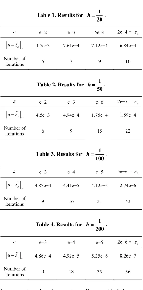
Tables 1-4 show, for different values of the

discretiza-tion parameter h, the error between the cubic spline

col-location S_ and the true solution u. We note the

con-vergence of the solution S_ to the function u depends

on the discretization parameter h and the penalty

pa-rameter . Theorem 6 implies that for a fixed h, this

convergence is guaranteed only if there exists h0 such that   h. Some experimental values of h are

given in Tables 1-4.

Theorems 1 and 6 imply that we have the error esti-mate between the exact solution and the discret penalty

solution is given by _{u S kh}2

 _ 

    . The obtained

[image:5.595.309.538.73.538.2]

results show the convergence of the discret penalty solu-tion to the solusolu-tion of the original obstacle problem as

Table 1. Results for = 1 20

h .

 e−2 e−3 5e−4 2e−4 = h

uS_ 4.7e−3 7.61e−4 7.12e−4 6.84e−4 Number of

iterations 5 7 9 10

Table 2. Results for = 1 50

h .

 e−2 e−3 e−6 2e−5 = h

uS_ 4.5e−3 4.94e−4 1.75e−4 1.59e−4 Number of

iterations 6 9 15 22

Table 3. Results for = 1 100

h .

 e−3 e−4 e−5 5e−6 = h

uS_ 4.87e−4 4.41e−5 4.12e−6 2.74e−6 Number of

iterations 9 16 31 43

Table 4. Results for = 1 200

h .

 e−3 e−4 e−5 2e−6 = h

uS 4.86e−4 4.92e−5 5.25e−6 8.26e−7 Number of

iterations 9 18 35 56

the parameters h and  get smaller provided they

sat-isfy the relation (21). Moreover, the numerical error

es-timates behave like which confirms what we

were expecting.

2

kh



7. Concluding Remarks

. The obtained numerical results show the

conver-gence of the approximate penalty solutions to the exact one and confirm the error estimates provided in this pa-per.



REFERENCES

[1] R. Glowinski, J. L. Lions and R. Trémolières, “Numerical Analysis of Variational Inequalities,” 8th Edition, North- Holland, Amsterdam, 1981.

[2] D. Kinderlehrer and G. Stampacchia, “An Introduction to Variational Inequalities and Their Applications,” Aca-demic Press, Inc., New York, 1980.

[3] R. P. Agarwal and C. S. Ryoo, “Numerical Verifications of Solutions for Obstacle Problems,” Computing Supple-menta, Vol. 15, 2001, pp. 9-19.

[4] R. Glowinski, Y.A. Kuznetsov and T-W. Pan, “A Pen-alty/Newton/Conjugate Gradient Method for the Solution of Obstacle Problems,” Comptes Rendus Mathematique, Vol. 336, No. 5, 2003, pp. 435-440.

[5] H. Huang, W. Han and J. Zhou, “The Regularization Method for an Obstacle Problem,” Numerische Mathe-matik, Vol. 69, No. 2, 1994, pp. 155-166.

doi:10.1007/s002110050086

[6] R. Scholz, “Numerical Solution of the Obstacle Problem by the Penalty Method,” Computing, Vol. 32, No. 4, 1984,

pp. 297-306. doi:10.1007/BF02243774

[7] H. Lewy and G. Stampacchia, “On the Regularity of the Solution of the Variational Inequalities,” Communica-tions on Pure and Applied Mathematics, Vol. 22, No. 2,

1969, pp. 153-188. doi:10.1002/cpa.3160220203

[8] X. Chen, “A Verification Method for Solutions of Non- smooth Equations,” Computing, Vol. 58, No. 3, 1997, pp.

281-294. doi:10.1007/BF02684394

[9] X. Chen, Z. Nashed and L. Qi, “Smooting Methods and

Semismooth Methods for Nondifferentiable Operator Equations,” SIAM Journal on Numerical Analysis, Vol. 38, No. 4, 2000, pp. 1200-1216.

doi:10.1137/S0036142999356719

[10] M.J. Śmietański, “A Generalizd Jacobian Based Newton Method for Semismooth Block-Triangular System of Equa- tions,” Journal of Computational and Applied Mathema- tics, Vol. 205, No. 1, 2007, pp. 305-313.

doi:10.1016/j.cam.2006.05.003

[11] H. N. Çaglar, S. H. Çaglar and E. H. Twizell, “The Nu-merical Solution of Fifth-Order Boundary Value Prob-lems with Sixth-Degree B-Spline Functions,” Applied Mathematics Letters, Vol. 12, No. 5, 1999, pp. 25-30.

doi:10.1016/S0893-9659(99)00052-X

[12] A. Lamnii, H. Mraoui, D. Sbibih, A. Tijini and A. Zidna, “Sextic Spline Collocation Methods for Nonlinear Fifth- Order Boundary Value Problems,” International Journal of Computer Mathematics, Vol. 88, No. 10, 2011, pp.

2072-2088. doi:10.1080/00207160.2010.519384

[13] C. de Boor, “A Practical Guide to Splines,” Springer Verlag, New York, 1994.

[14] R. R. Phelps, “Convex Functions, Monotone Operators and Differentiability (Lecture Notes in Mathematics),” Springer, New York 1993.

[15] F. H. Clarke, “Optimization and Nonsmooth Analysis,” Wiley, New York, 1993.

[16] L. Qi, “Convergence Analysis of Some Algorithms for Solving Some Nonsmooth Equations,” Mathematics of Operations Research, Vol. 18, No. 1, 1993, pp. 227-244.

doi:10.1287/moor.18.1.227

[17] L. Qi and J. Sun, “A Nonsmooth Version of the New-thon’s Method,” Mathematical Programming, Vol. 58,

No. 1-3, 1993, pp. 353-367. doi:10.1007/BF01581275 [18] J. S. Pang and L. Qi, “Nonsmooth Functions: Motivation

and Algorithms,” SIAM Journal on Optimization, Vol. 3,