The 2 Extra Diagnosability of Alternating Group Graphs under the PMC Model and MM* Model

http://www.scirp.org/journal/ajcm ISSN Online: 2161-1211

ISSN Print: 2161-1203

DOI: 10.4236/ajcm.2018.81004 Mar. 12, 2018 42 American Journal of Computational Mathematics

The 2-Extra Diagnosability of Alternating

Group Graphs under the PMC Model

and MM* Model

Shiying Wang, Yunxia Ren

School of Mathematics and Information Science, Henan Normal University, Xinxiang, China

Abstract

Diagnosability of a multiprocessor system is one important study topic. In 2015, Zhang et al. proposed a new measure for fault diagnosis of the system, namely, g-extra diagnosability, which restrains that every fault-free compo-nent has at least

(

g+1

)

fault-free nodes. As a favorable topology structure

of interconnection networks, the n-dimensional alternating group graph AGn has many good properties. In this paper, we give that the 2-extra diagnosabil-ity of AGn is 6n−17 for n≥5 under the PMC model and MM* model.

Keywords

Interconnection Network, Diagnosability, Alternating Group Graph

1. Introduction

Many multiprocessor systems take interconnection networks (networks for short) as underlying topologies and a network is usually represented by a graph where nodes represent processors and links represent communication links be-tween processors. We use graphs and networks interchangeably. For a multi-processor system, study on the topological properties of its network is impor-tant. Furthermore, some processors may fail in the system, so processor fault identification plays an important role for reliable computing. The first step to deal with faults is to identify the faulty processors from the fault-free ones. The identification process is called the diagnosis of the system. A system is said to be t-diagnosable if all faulty processors can be identified without replacement, pro-vided that the number of faults presented does not exceed t. The diagnosability of a system G is the maximum value of t such that G is t-diagnosable [1][2][3]. For a How to cite this paper: Wang, S.Y. and

Ren, Y.X. (2018) The 2-Extra Diagnosabili-ty of Alternating Group Graphs under the PMC Model and MM* Model. American Journal of Computational Mathematics, 8, 42-54.

https://doi.org/10.4236/ajcm.2018.81004

Received: January 25, 2018 Accepted: March 9, 2018 Published: March 12, 2018

Copyright © 2018 by authors and Scientific Research Publishing Inc. This work is licensed under the Creative Commons Attribution International License (CC BY 4.0).

http://creativecommons.org/licenses/by/4.0/

DOI: 10.4236/ajcm.2018.81004 43 American Journal of Computational Mathematics t-diagnosable system, Dahbura and Masson [1] proposed an algorithm with time complex _{O n}

( )

2.5 , which can effectively identify the set of faulty processors.

Several diagnosis models were proposed to identify the faulty processors. One major approach is the Preparata, Metze, and Chien’s (PMC) diagnosis model in-troduced by Preparata et al.[4]. The diagnosis of the system is achieved through two linked processors testing each other. Another major approach, namely the comparison diagnosis model (MM model), was proposed by Maeng and Malek [5]. In the MM model, to diagnose a system, a node sends the same task to two of its neighbors, and then compares their responses. In 2005, Lai et al.[3] intro-duced a restricted diagnosability of multiprocessor systems called conditional diagnosability. They consider the situation that any fault set cannot contain all the neighbors of any vertex in a system. In 2012, Peng et al. [6] proposed a measure for fault diagnosis of the system, namely, g-good-neighbor diagnosabil-ity (which is also called g-good-neighbor conditional diagnosability), which re-quires that every fault-free node has at least g fault-free neighbors. In [6], they studied the g-good-neighbor diagnosability of the n-dimensional hypercube un-der the PMC model. In [7], Wang and Han studied the g-good-neighbor diag-nosability of the n-dimensional hypercube under the MM* model. Yuan et al.[8] and [9] studied that the g-good-neighbor diagnosability of the k-ary n-cube

(

k≥3

)

under the PMC model and MM* model. The Cayley graph CΓn gen-erated by the transposition tree Γn has recently received considerable atten-tion. In [10] [11], Wang et al. studied the g-good-neighbor diagnosability of

n

CΓ under the PMC model and MM* model for g=1,2. In 2015, Zhang et al.

[12] proposed a new measure for fault diagnosis of the system, namely, g-extra diagnosability, which restrains that every fault-free component has at least

(

g+1

)

fault-free nodes. In [12], they studied the g-extra diagnosability of the n-dimensional hypercube under the PMC model and MM* model. The n-dimensional bubble-sort star graph BSn has many good properties. In 2016, Wang et al.[13] studied the 2-extra diagnosability of BSn under the PMC model and MM* model.

As a favorable topology structure of interconnection networks, the n-dimensional alternating group graph AGn has many good properties. In this paper, we give that the 2-extra diagnosability of AGn is 6n−17 for n≥5 under the PMC model and MM* model.

2. Preliminaries

In this section, some definitions and notations needed for our discussion, the al-ternating group graph, the PMC model and the MM* model are introduced.

2.1. Notations

A multiprocessor system is modeled as an undirected simple graph G=

(

V E,

)

,

whose vertices (nodes) represent processors and edges (links) represent com-munication links. Given a nonempty vertex subset V′ of V, the induced sub-graph by V′ in G, denoted by G V

[ ]

′ , is a graph, whose vertex set is V′ and

de-DOI: 10.4236/ajcm.2018.81004 44 American Journal of Computational Mathematics gree dG

( )

v of a vertex v is the number of edges incident with v. The minimum degree of a vertex in G is denoted by δ

( )

G . For any vertex v, we define the

neighborhood NG

( )

v of v in G to be the set of vertices adjacent to v. u is called a neighbor vertex or a neighbor of v for u∈NG

( )

v . Let S⊆V . We use

( )

G

N S to denote the set



v S∈ NG

( )

v \S. For neighborhoods and degrees, we

will usually omit the subscript for the graph when no confusion arises. A graph G is said to be k-regular if for any vertex v, dG

( )

v =k. The connectivity κ

( )

G of a graph G is the minimum number of vertices whose removal results in a dis-connected graph or only one vertex left when G is complete. Let F1 and F2

be two distinct subsets of V, and let the symmetric difference

(

) (

)

1 2 1\ 2 2\ 1

F F∆ = F F  F F . Let B1,,Bk

(

k≥2

)

be the components of

1

G−F . If V B

( )

1 ≤≤V B

( )

k

(

k≥2

)

, then Bk is called the maximum component of G−F1. For graph-theoretical terminology and notation not

de-fined here we follow [14].

Let G=

(

V E,

)

. A fault set F⊆V is called a g-good-neighbor faulty set if

( ) (

\

)

N v  V F ≥g for every vertex v in V \F. A g-good-neighbor cut of G is a g-good-neighbor faulty set F such that G−F is disconnected. The minimum cardinality of g-good-neighbor cuts is said to be the g-good-neighbor connectiv-ity of G, denoted by ( )g

( )

G

κ . A fault set F ⊆V is called a g-extra faulty set if

every component of G−F has at least

(

g+1

)

vertices. A g-extra cut of G is a

g-extra faulty set F such that G−F is disconnected. The minimum cardinality of g-extra cuts is said to be the g-extra connectivity of G, denoted by ( )g

( )

G

κ . Proposition 2.1 [15]Let G be a connected graph. Then ( )g

_{( )}

( )g

_{( )}

G G

κ ≤κ . Proposition 2.2 [15]Let G be a connected graph. Then ( )1

( )

( )1

( )

G G

κ =κ .

2.2. The PMC Model and the MM

*

Model

Under the PMC model [5][8], to diagnose a system G, two adjacent nodes in G are capable to perform tests on each other. For two adjacent nodes u and v in

( )

V G , the test performed by u on v is represented by the ordered pair

( )

u v, .

The outcome of a test

( )

u v, is 1 (resp. 0) if u evaluate v as faulty (resp.

fault-free). We assume that the testing result is reliable (resp. unreliable) if the node u is fault-free (resp. faulty). A test assignment T for G is a collection of tests for every adjacent pair of vertices. It can be modeled as a directed testing graph T =

(

V G

( )

,L

)

, where

( )

u v, ∈L implies that u and v are adjacent in G.

The collection of all test results for a test assignment T is called a syndrome. Formally, a syndrome is a function σ:L

{ }

0,1 . The set of all faulty

proces-sors in G is called a faulty set. This can be any subset of V G

( )

. For a given

syn-drome σ, a subset of vertices F⊆V G

( )

is said to be consistent with σ if

syn-drome σ can be produced from the situation that, for any

( )

u v, ∈L such that

\

u V∈ F,

σ

( )

u v, = 1 if and only if v∈F. This means that F is a possible set of faulty processors. Since a test outcome produced by a faulty processor is unre-liable, a given set F of faulty vertices may produce a lot of different syndromes. On the other hand, different faulty sets may produce the same syndrome. Let

( )

F

DOI: 10.4236/ajcm.2018.81004 45 American Journal of Computational Mathematics PMC model, two distinct sets F1 and F2 in V G

( )

are said to be

indistin-guishable if σ

( )

F1 σ

( )

F 2≠ ∅, otherwise, F1 and F2 are said to be

distin-guishable. Besides, we say

(

F F1, 2

)

is an indistinguishable pair if

( )

F1

( )

F 2

σ _σ ≠ ∅_{; else,}

(

F F₁, ₂

)

is a distinguishable pair.

Using the MM model, the diagnosis is carried out by sending the same test-ing task to a pair of processors and compartest-ing their responses. We always as-sume the output of a comparison performed by a faulty processor is unreliable. The comparison scheme of a system G=

(

V E,

)

is modeled as a multigraph,

denoted by M V G

(

( )

,L

)

, where L is the labeled-edge set. A labeled edge

( )

u v, _w∈L represents a comparison in which two vertices u and v are

com-pared by a vertex w, which implies uw vw, ∈E G

( )

. The collection of all

com-parison results in M V G

(

( )

,L

)

is called the syndrome, denoted by σ*, of the diagnosis. If the comparison

( )

u v, _w disagrees, then *

(

( )

)

, _w 1

u v

σ = . oth-erwise, *

(

( )

_,

)

₀

w

u v

σ = . Hence, a syndrome is a function from L to

{ }

0,1 .

The MM* model is a special case of the MM model. In the MM* model, all comparisons of G are in the comparison scheme of G, i.e., if uw vw, ∈E G

( )

,

then

( )

u v, _w∈L. Similar to the PMC model, we can define a subset of vertices

( )

F ⊆V G is consistent with a given syndrome

σ

* _{and two distinct sets} 1 F

and F2 in V G

( )

are indistinguishable (resp. distinguishable) under the

MM* model.

A system G=

(

V E,

)

is g-good-neighbor t-diagnosable if F₁ and F2 are

distinguishable for each distinct pair of g-good-neighbor faulty subsets F1 and

2

F of V with F1 ≤t and F2 ≤t . The g-good-neighbor diagnosability

( )

g

t G of G is the maximum value of t such that G is g-good-neighbor

t-diagnosable.

Proposition 2.3 ([6]) For any given system G, tg

( )

G ≤tg′

( )

G if g≤g′. In a system G=

(

V E,

)

, a faulty set F⊆V is called a conditional faulty set

if it does not contain all the neighbor vertices of any vertex in G. A system G is conditional t-diagnosable if every two distinct conditional faulty subsets

1, 2

F F ⊆V with F1 ≤t F, 2 ≤t, are distinguishable. The conditional

diagnosa-bility t Gc

( )

of G is the maximum number of t such that G is conditional t-diagnosable. By [16], t Gc

( ) ( )

≥t G .

Theorem 2.4 [10] For a system G=

(

V E,

)

, t G

( )

=t G0

( ) ( )

≤t G1 ≤t Gc

( )

. In [10], Wang et al. proved that the 1-good-neighbor diagnosability of the Bubble-sort graph Bn under the PMC model is 2n−3 for n≥4. In [17], Zhou et al. proved the conditional diagnosability of Bn is 4n−11 for n≥4 under the PMC model. Therefore, t G1

( )

<t Gc

( )

when n≥5 and

( )

( )

1 c

t G =t G when n=4.

In a system G=

(

V E,

)

, a faulty set F⊆V is called a g-extra faulty set if

every component of G−F has more than g nodes. G is g-extra t -diagnosable if and only if for each pair of distinct faulty g-extra vertex subsets

( )

1, 2

F F ⊆V G such that Fi ≤t, F1 and F2 are distinguishable. The g-extra

DOI: 10.4236/ajcm.2018.81004 46 American Journal of Computational Mathematics g-extra t-diagnosable.

Proposition 2.5 [13] For any given system G, tg

( )

G ≤tg′

( )

G if g≤g′. Theorem 2.6 [13] For a system G=

(

V E,

)

, t G

( )

=t G0

( )

≤tg

( )

G ≤tg

( )

G . Theorem 2.7 [13] For a system G=

(

V E,

)

, t G₁

( )

=t G₁

( )

.

2.3. Alternating Group Graph

In this section, we give the definition and some properties of the alternating group graph. In the permutation

1 2

1 2

n

n

p p p

 

 

 



 , i→pi. For the

conveni-ence, we denote the permutation

1 2

1 2

n

n

p p p

 

 

 



 by p p1 2pn. Every permutation can be denoted by a product of cycles [18]. For example,

( )

1 2 3 132 3 1 2

 ₌

 

  . Specially,

( )

1 2 1 1 2 n n  ₌     

 . The product στ of two

permutations is the composition function τ followed by σ, that is,

( )( ) ( )

12 13 = 132 . For terminology and notation not defined here we follow [18].

Let

[ ]

n =

{

1, 2,,n

}

, and let S_n be the symmetric group on

[ ]

n containing

all permutations p= p p1 2pn of

[ ]

n . The alternating group An is the sub-group of Sn containing all even permutations. It is well known that

( ) ( )

{

12 , 1 2 ,3i i ≤ ≤i n

}

is a generating set for An. The n-dimensional alternat-ing group graph AGn is the graph with vertex set V AG

(

n

)

=An in which two vertices u, v are adjacent if and only if u=v

( )

12i or u=v i

( )

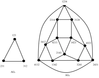
1 2 , 3≤ ≤i n. The identity element of An is (1). The graphs AG3 and AG4 are depicted in

Figure 1. It is easy to see from the definition that AGn is a 2

(

n−2

)

-regular graph on n! 2 vertices.

As a favorable topology structure of interconnection networks, alternating group graphs have been shown to have many desirable properties such as strong hierarchy, high connectivity, small diameter and average distance, etc. For de-tails, see [19] for a comparison of the hypercube, the star graph and the alter-nating group graph.

Theorem 2.8 ([19]) AGn is vertex transitive and edge transitive. Theorem 2.9 ([20]) ( )2

(

)

6 19 n

AG n

κ = − for n≥5.

We can partition AGn into n subgraphs

1 2

, , , n

n n n

AG AG  AG , where every

vertex u=x x1 2xn∈V AG

(

n

)

has a fixed integer i in the last position xn for

[ ]

i∈ n . It is obvious that AGni is isomorphic to AGn−1 for i∈

[ ]

n .

Proposition 2.10 [20] Let i n

AG be defined as above. Then there are

(

n−2 !

)

independent cross-edges between two different i n

AG ‘s.

Proposition 2.11 [8]

κ

(

AGn

)

=

δ

(

AGn

)

=2n−4 for n≥3. Furthermore,

n

AG is tightly hyper connected for n≥4, that is to say, each minimum vertex cut creates exactly two components, one of which is an isolated vertex.

Proposition 2.12 ([20]) Let F be a vertex-cut of AGn (n≥5) such that

6 20

F ≤ n− . Then, AGn−F satisfies one of the following conditions:

[image:6.595.212.539.72.328.2]

DOI: 10.4236/ajcm.2018.81004 47 American Journal of Computational Mathematics

Figure 1. AGn for n = 3, 4.

edge;

2) AGn−F has three components, two of which are isolated vertices.

Proposition 2.13 ([20]) Let F be a vertex-cut of AGn (n≥5) such that

6 19

F ≤ n− . Then, AG_n−F satisfies one of the following conditions:

1) AGn−F has two components, one of which is an isolated vertex, an edge or a path of length 2;

2) AGn−F has three components, two of which are isolated vertices. Proposition 2.14 [20] For

(

r

)

n

u∈V AG ,

( )

i n

u+∈V AG ,

(

j

)

n

u−∈V AG for 4

n≥ and i≠ j.

Lemma 2.15 ([21]) Any 4-cycle in AGn has the form u u u u u1 2 3 4 1 where

( )

2 1 12

u =u i , u3=u2

( )

12j , u4=u3

( )

12i , u1=u4

( )

12j for some i j, with i≠ j.

3. The 2-Extra Diagnosability of Alternating Group Graphs

under the PMC Model

In this section, we will give 2-extra diagnosability of alternating group graph networks under the PMC model.

Theorem 3.1 ([8]) A system G=

(

V E,

)

is g-extra t-diagnosable under the

PMC model if and only if there is an edge uv∈E with u∈V\

(

F₁F₂

)

and

1 2

v∈ ∆F F for each distinct pair of g-extra faulty subsets F1 and F2 of V with

1

F ≤t and F2 ≤t.

Lemma 3.2 Let A=

{

( ) ( ) ( )

1 , 132 , 142

}

, n≥4 and let F1=NAG_n

( )

A ,

( )

2 AGn

F =AN A . Then F1 =6n−19, F2 =6n−16, F1 is a 2-extra cut of

n

DOI: 10.4236/ajcm.2018.81004 48 American Journal of Computational Mathematics Proof. By A=

{

( ) ( ) ( )

1 , 132 , 142

}

, we have that AG An

[ ]

is a path

( )

132 ,

( )

1 ,

( )

142 . Suppose n=4. Then N A

( ) {

= 2314, 4132,1423, 4321,3241

}

=5 (see Figure 1). We prove this lemma (part) by induction on n. The result holds for n=4. Assume n≥5 and the result holds for AG_n−1, i.e.,

(

)

1 6 1 19 6 25

F = n− − = n− . We decompose AGn into n sub-alternating group graph, 1 2

, , , n

n n n

AG AG  AG , where each AGni has a fixed i in the last position of the label strings which represents the vertices and is isomorphic to AGn−1. Note

that

( )

( )

1

{

( ) ( )( ) ( )( )

}

12 ), 1 23 , 1 24 3

n

N A V AG = n n n = ,

( )

(

2

)

{

( )

}

1 2 1

n

N A V AG = n = , N A

( )

V AG

( )

n3 =

{

(

2 3n

)

}

=1,

( )

(

4

)

{

(

)

}

2 4 1

n

N A V AG = n = and

( )

( )

i 0

n

N A V AG = for i=5,,n−1. Therefore, F1 =6n−25 6+ =6n−19 and F2 =6n−16.

Let *

( )

1

i

i n

F =FV AG for i∈

{

1, 2,,n

}

. Note that 4 2 1342, 2143, 4213,3412,1342

AG −F = is a 4-cycle. We prove this lemma (part)

by induction on n. The result holds for n=4. Assume n≥5 and the result holds for AGn−1, i.e., F1 is a 2-extra cut of AGn−1, and AGn−1−F1 has two

components AGn−1−F2 and AGn−1

[ ]

A . Since

( )

( )

1

{

( ) ( )( ) ( )( )

}

12 , 1 23 , 1 24 3

n

N A V AG = n n n = ,

( )

(

2

)

{

( )

}

1 2 1

n

N A V AG = n = , N A

( )

V AG

( )

n3 =

{

(

2 3n

)

}

=1,

( )

(

4

)

{

(

)

}

2 4 1

n

N A V AG = n = and N A

( )

V AG

( )

ni =0 for i=5,,n−1,

by Propositions 2.10 and 2.11,

(

2 *

) (

3 *

)

(

*

)

2 3

n

n n n n n

AG V AG_ −F V AG −F V AG −F _ is connected for

5

n≥ . By inductive hypothesis, AG_n−1−F₂ is connected. Since

( )

* 1

i

i n

F =FV AG , by Proposition 2.14,

(

N x

( )

V AG

( )

_ni

)

F_i*= ∅ for

(

n 1 2

)

x V AG∈ ₋ −F . Therefore,

(

1

) (

2 *

) (

3 *

)

(

*

)

2 2 3 2

n

n n n n n n n

AG V AG_ −F V AG −F V AG −F V AG −F _=AG −F is connected. Note that V AG

(

n−F2

)

≥3 and V AG A

(

n

[ ]

)

=3. Therefore,

1

F is a 2-extra cut of AGn, and AGn−F1 has two components AGn−F2

and AG An

[ ]

. The proof is complete.

A connected graph G is super g-extra connected if every minimum g-extra cut F of G isolates one connected subgraph of order g+1. If, in addition, G−F has two components, one of which is the connected subgraph of order g+1,

then G is tightly super g-extra connected.

Corollary 3.3 Let n≥5. Then AGn is tightly

(

6n−19

)

super 2-extra connected.

Proof. Let F1⊆An. By Lemma 3.2, there is one F1 =6n−19 such that F is a

2-extra cut of AGn. Let F be a minimum 2-extra cut of AGn (n≥5). Then

1

F ≤ F . Suppose that F ≤6n−20. By Lemma 3.3, F is not a 2-extra cut of

n

AG . Therefore, F = 6n−19. Since F is a 2-extra cut of AG_n, by Lemma 2.14,

n

AG −F has two components, one of which is a path of order 3. The proof is

complete.

DOI: 10.4236/ajcm.2018.81004 49 American Journal of Computational Mathematics Proof. Let A=

{

( ) ( ) ( )

1 , 132 , 142

}

, and let F1=NAGn

( )

A , F2=ANAGn

( )

A .

By Lemma 3.2, F1 =6n−19, F2 =6n−16, F1 is a 2-extra cut of AGn, and

1

n

AG −F has two components AGn−F2 and AG An

[ ]

. Therefore, F1 and

2

F are both 2-extra faulty sets of AGn with F1 =6n−19 and F2 =6n−16.

Since A= ∆F F1 2 and NAGn

( )

A =F1⊂F2, there is no edge of AGn between

(

n

) (

\ 1 2

)

V AG FF and F F₁∆ ₂. By Theorem 3.1, we can deduce that AGn is not 2-extra (6n−16)-diagnosable under PMC model. Hence, by the definition

of 2-extra diagnosability, we conclude that the 2-extra diagnosability of AGn is less than 6n−16, i.e., t₂

(

AG_n

)

≤6n−17. The proof is complete.

Lemma 3.5 Let n≥5. Then the 2-extra of the n-dimensional alternating group graph AGn under the PMC model, t2

(

AGn

)

≥6n−17.

Proof. By the definition of 2-extra diagnosability, it is sufficient to show that

n

AG is 2-extra

(

6n−17

)

-diagnosable. By Theorem 3.1, to prove AG_n is

2-extra

(

6n−17

)

-diagnosable, it is equivalent to prove that there is an edge

(

n

)

uv∈E AG with u∈V AG

(

n

) (

\ F1F2

)

and v∈ ∆F F1 2 for each distinct

pair of 2-extra faulty subsets F1 and F2 of V AG

(

n

)

with F1 ≤6n−17 and

2 6 17

F ≤ n− .

We prove this statement by contradiction. Suppose that there are two distinct 2-extra faulty subsets F1 and F2 of AGn with F1 ≤6n−17 and

2 6 17

F ≤ n− , but the vertex set pair

(

F F1, 2

)

is not satisfied with the condition

in Theorem 3.1, i.e., there are no edges between V AG

(

n

) (

\ F1F2

)

and F F1∆ 2.

Without loss of generality, assume that F2\F1≠ ∅. Assume V AG

(

n

)

=F1F2.

By the definition of An, F1F2 = An =n! 2. We claim that n! 2>12n−34 for n≥5 , i.e., n!>24n−68 for n≥5 . When n=5 , n! 120= ,

24n−68=52. So n!>24n−68 for n=5. Assume that n!>24n−68 for 5

n≥ .

(

n+1 !

)

=n n!

(

+ >1

) (

n+1 24

)(

n−68

) (

=n 24n−68

) (

+ 24n−44

)

−24=

(

)

(

)

(

)

(

2

)

24 n+ −1 68 +n 24n−68 −24= 24 n+ −1 68 +4 6n −17n−6

   

    . It is

suf-ficient to show that 2

6n −17n− ≥6 0 for n≥5. Let y=6x2−17x−6. Then

2

6 17 6

y= x − x− is a quadratic function. When x≥5, y=6x2−17x− ≥6 0.

Since n≥5, we have that n! 2=V AG

(

_n

)

= F₁F₂ = F₁ + F₂ − F₁F₂ ≤

(

)

1 2 2 6 17 12 34

F + F ≤ n− = n− , a contradiction to n! 2>12n−34. Therefore,

let V AG

(

n

)

≠F1F2 as follows.

Since there are no edges between V AG

(

n

) (

\ F1F2

)

and F F1∆ 2, and F1 is

a 2-extra faulty set, AGn−F1 has two parts AGn− −F1 F2 and AG Fn

[

2\F1

]

(for convenience). Thus, every component Gi of AGn− −F1 F2 has

( )

_i 3

V G ≥ and every component B_i′ of AG Fn

[

2\F1

]

has V B

( )

i′ ≥3. Simi-larly, every component Bi′′ of AG F Fn

[

1\ 2

]

has V B

( )

′′ ≥3 when

1\ 2

F F ≠ ∅. Therefore, F1∩F2 is also a 2-extra faulty set of AGn. Note that

1 2 1

F F =F is also a 2-extra faulty set when F F1\ 2= ∅. Since there are no

edges between V AG

(

n− −F1 F2

)

and F F1∆ 2, F1F2 is a 2-extra cut of AGn. If F1F2= ∅, this is a contradiction to that AGn is connected. Therefore,

1 2

F F ≠ ∅ . Since n≥5, by Theorem 2.9, F₁F₂ ≥6n−19 . Therefore,

2 2\ 1 1 2 3 6 19 6 16

DOI: 10.4236/ajcm.2018.81004 50 American Journal of Computational Mathematics

2 6 17

F ≤ n− . So AGn is 2-extra

(

6n−17

)

-diagnosable. By the definition of

(

)

2 n

t AG , t2

(

AGn

)

≥6n−17. The proof is complete.

Combining Lemma 3.4 and 3.5, we have the following theorem.

Theorem 3.6 Let n≥5. Then the 2-extra diagnosability of the n-dimensional alternating group graph AGn under the PMC model is 6n−17.

4. The 2-Extra Diagnosability of Alternating Group Graphs

under the MM* Model

Before discussing the 2-extra diagnosability of the n-dimensional alternating group graph AGn under the MM* model, we first give a theorem.

Theorem 4.1 ([1][18]) A system G=

(

V E,

)

is g-extra t-diagnosable under

the MM* model if and only if for each distinct pair of g-extra faulty subsets F1

and F2 of V with F1 ≤t and F2 ≤t satisfies one of the following

condi-tions.

1) There are two vertices u w V, ∈ \

(

F1F2

)

and there is a vertex v∈ ∆F F1 2

such that uw∈E and vw∈E.

2) There are two vertices u v, ∈F1\F2 and there is a vertex w V∈ \

(

F1F2

)

such that uw∈E and vw∈E.

3) There are two vertices u v, ∈F2\F1 and there is a vertex w V∈ \

(

F1F2

)

such that uw∈E and vw∈E.

Lemma 4.2 Let n≥5. Then the 2-extra diagnosability of the n-dimensional alternating group graph AGn under the MM* model, t2

(

AGn

)

≤6n−17.

Proof. Let A=

{

( ) ( ) ( )

1 , 132 , 142

}

, and let ₁

( )

n

AG

F =N A , ₂

( )

n

AG

F =AN A .

By Lemma 3.2, F1 =6n−19, F2 =6n−16, F1 is a 2-extra cut of AGn, and

1

n

AG −F has two components AG_n−F₂ and AGn

[ ]

A . Therefore, F1 and

2

F are both 2-extra faulty sets of AGn with F1 =6n−19 and F2 =6n−16.

By the definitions of F1 and F2, F F1∆ =2 A. Note F F1\ 2 = ∅, F2\F1=A

and

(

V AG

(

n

) (

\ F1F2

)

)

A= ∅. Therefore, both F1 and F2 are not

satis-fied with any one condition in Theorem 4.1, and AGn is not 2-extra

(

6n−16

)

diagnosable. Hence, t2

(

AGn

)

≤6n−17. Thus, the proof is complete.

A component of a graph G is odd according as it has an odd number of ver-tices. We denote by o G

( )

the number of add component of G.

Lemma 4.3 ([13] Tutte’s Theorem) A graph G=

(

V E,

)

has a perfect

matching if and only if o G

(

−S

)

≤ S for all S⊆V.

Lemma 4.4 Let n≥4. Then AG_n has a perfect matching.

Proof. Note that a perfect matching of AG4 is

{

[

1342, 4132 , 2431,1234 ,

]

[

]

[

3241, 4321 , 1423,3124 , 3412, 2314 , 2143, 4213

] [

] [

] [

]

}

(see Figure 1). We prove this lemma by induction on n. The result holds for n=4. Assume n≥5 and the result holds for AGn−1, i.e., AGn−1 has a perfect matching. We decompose

n

AG into n sub-alternating group graph, AG AGn1, n2,,AGnn, where each i n

AG

has a fixed i in the last position of the label strings which represents the vertices and is isomorphic to AGn−1. Therefore,

i n

AG has a perfect matching. Let Mi be a perfect matching of i

n

DOI: 10.4236/ajcm.2018.81004 51 American Journal of Computational Mathematics n

AG . The proof is complete.

Lemma 4.5 Let n≥5. Then the 2-extra diagnosability of the n-dimensional alternating group graph AGn under the MM* model, t2

(

AGn

)

≥6n−17.

Proof. By the definition of 2-extra diagnosability, it is sufficient to show that n

AG is 2-extra

(

6n−17

)

-diagnosable.

Suppose, on the contrary, that there are two distinct 2-extra faulty subsets F1

and F2 of AGn with F1 ≤6n−17 and F2 ≤6n−17, but the vertex set pair

(

F F1, 2

)

is not satisfied with any one condition in Theorem 4.1. Without loss of generality, assume that F2\F1≠ ∅. Assume V AG

(

n

)

=F1F2. By the

defini-tion of An, F1F2 = An =n! 2. Similar to the discussion on

(

n

)

1 2

V AG ≠FF in Lemma 3.5, we can deduce V AG

(

n

)

=F1F2. Therefore,

(

n

)

1 2

V AG ≠FF .

Claim 1. AGn− −F1 F2 has no isolated vertex.

Suppose, on the contrary, that AGn− −F1 F2 has at least one isolated vertex

1

w . Since F1 is one 2-extra faulty set, there is a vertex u∈F2\F1 such that u

is adjacent to w1. Meanwhile, since the vertex set pair

(

F F1, 2

)

is not satisfied

with any one condition in Theorem 4.1, by the condition (3) of Theorem 4.1, there is at most one vertex u∈F2\F1 such that u is adjacent to w1. Thus,

there is just a vertex u∈F2\F1 such that u is adjacent to w1. If F F1\ 2= ∅,

then F1⊆F2 . Since F2 is a 2-extra faulty set, every component Gi of

1 2 2

n n

AG − −F F =AG −F has V G

( )

i ≥3. Therefore, AGn− −F1 F2 has no

isolated vertex. Thus, let F1\F2≠ ∅. Similarly, we can deduce that there is just

a vertex a∈F1\F2 such that a is adjacent to w1. Let W ⊆An\

(

F1F2

)

be

the set of isolated vertices in AGnAn\

(

F1F2

)

, and let H be the induced subgraph by the vertex set An\

(

F1 F2 W

)

. Then for any w W∈ , there are

(

2n−6

)

neighbors in F₁F₂.

By Lemmas 4.3 and 4.4, W ≤o AG

(

n−

(

F1F2

)

)

≤ F1F2 = F1 + F2 −

(

) (

)

1 2 2 6 17 2 6 10 28

F F ≤ n− − n− = n− . Since n≥5 , n! 4>10n−28 .

Therefore, W ≤n! 4. Suppose V H

( )

= ∅. Then n! 2=V AG

(

n

)

= F1F2 +

(

) (

)

1 2 1 2 2 6 17 2 6 10 28 ! 4

W = F + F − F F +W ≤ n− − n− +W = n− +W <n

10n 28

+ − _{and hence} n! 4<10n−28, a contradiction to that n≥5. So

( )

V H ≠ ∅.

Since the vertex set pair

(

F F1, 2

)

is not satisfied with the condition (1) of

Theorem 4.1, and any vertex of V H

( )

is not isolated in H, we induce that there

is no edge between V H

( )

and F F1∆ 2. Thus, F1 is a vertex cut of AGn. Since

1

F is a 2-extra faulty set of AGn, we have that every component Hi of H has

( )

_i 3

V H ≥ and every component Bi of AG Wn 

(

F2\F1

)

 has

( )

_i 3

V B ≥ . Therefore, F₁ is also a 2-extra cut of AGn. If F1F2= ∅, then

this is a contradiction to that AGn is connected. Therefore, F1F2≠ ∅. By

Theorem 2.9, F1 ≥6n−19. Since F1 ≤6n−17, we have

1

6n−19≤ F ≤6n−17. Since every component Bi of AG Wn 

(

F2\F1

)

 has

( )

_i 3

V B ≥ , we have F₂\F₁ ≥2 and hence F1 =6n−17 and F2\F1 =2.

DOI: 10.4236/ajcm.2018.81004 52 American Journal of Computational Mathematics

1\ 2

F F = ∅. Therefore, let F1\F2=/ ∅. Similarly, we can deduce that F2 is also

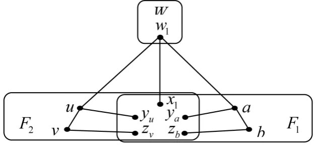
a 2-extra cut of AGn, F2 =6n−17 and F F1\ 2 =2 . Let F2\F1=

{ }

u v, ,

{ }

1\ 2 ,

F F = a b , and let vuw ab1 be a path in AGn (see Figure 2).

Since there is no edge between V H

( )

and F F₁∆ ₂ , V H

( )

≠ ∅ and

2\ 1

F F ≠ ∅, F1F2 is a cut of AGn. By the above result, F1F2 =6n−19.

Since every component Hi of H has V H

( )

i ≥3, every component Bi of

(

2\ 1

)

n

AG W_  F F _ has V B

( )

_i ≥3 and every component Bi′ of

(

2\ 1

)

n

AG W_  F F _ has V B

( )

_i′ ≥3, we have that every component H_i of H

has V H

( )

_i ≥3 and every component Gi of AG Wn 

(

F2\F1

) (

 F1\F2

)

 has V G

( )

_i ≥3. By Theorem 2.9, κ( )2

(

AG_n

)

=6n−19 and F₁∩F₂ is a

min-imum 2-extra cut of AGn. Therefore, F1F2 =6n−19. By Corollary 3.3,

n

AG is tightly

(

6n−19

)

super 2-extra connected, i.e., AGn−

(

F1F2

)

has

two components, one of which is the path of length 3. Since

2\ 1 1\ 2 5

F F + F F +W ≥ , we have that V AG

(

n− −F1 F2−W

)

=3. Thus,

(

)

(

1 2

)

2 1 1 2 2 1

! 2 _{n n} \ \ 3

n =V AG = V AG −F −F −W + F F + F F +W + F F < +

2+ +2 n! 4 6+ n−19=6n−12+n! 4 and hence n! 4<6n−12, a contradiction

to n≥5. The proof Claim 1 is complete.

Let u∈V AG

(

n

) (

\ F1F2

)

. By Claim 1, u has at least one neighbor in

1 2

n

AG − −F F . Since the vertex set pair

(

F F1, 2

)

is not satisfied with any one

condition in Theorem 4.1, by the condition (1) of Theorem 4.1, for any pair of adjacent vertices u w V AG, ∈

(

n

) (

\ F1F2

)

, there is no vertex v∈ ∆F F1 2 such

that uw∈E AG

(

n

)

and vw∈E AG

(

n

)

. It follows that u has no neighbor in

1 2

F F∆ . By the arbitrariness of u, there is no edge between V AG

(

n

) (

\ F1F2

)

and F F1∆ 2. Since F2\F1≠ ∅ and F1 is a 2-extra faulty set, every component

i

H of AGn− −F1 F2 has V H

( )

i ≥3 and every component Gi of

[

]

(

2\ 1

)

n

AG F F has V G

( )

_i ≥3. Suppose that F₁\F₂ =∅. Then F1F2=F1.

Since F1 is a 2-extra faulty set of AGn, we have that F1∩F2=F1 is a 2-extra

f a u l t y s e t o f AGn . S i n c e V AG

(

n− −F1 F2

)

= V AG

(

n−F2

)

≥3 a n d

2 1

|F \F | 3≥ , F1F2=F1 is a 2-extra cut of AGn. Suppose that F F1\ 2 ≠ ∅. If

1 2

[image:11.595.217.532.561.709.2]

F F = ∅, then this is a contradiction to that AGn is connected. Therefore,

DOI: 10.4236/ajcm.2018.81004 53 American Journal of Computational Mathematics

1 2

F F ≠ ∅. Similarly, every component Bi of AGn

(

[

F F1\ 2

]

)

has V B

( )

i ≥3. Therefore, F1F2 is a 2-extra cut of AGn . By Theorem 2.9, we have

1 2 6 19

F F ≥ n− . Therefore, F2 = F2\F1+ F1F2 ≥ +3

(

6n−19

)

=6n−16 ,

which contradicts F2 ≤6n−17. Therefore, AGn is 2-extra

(

6n−17

)

diagnosa-ble and t2

(

AGn

)

≥6n−17. The proof is complete.

Combining Lemma 4.2 and 4.5, we have the following theorem.

Theorem 4.6 Let n≥5. Then the 2-extra diagnosability of the the n-dimensional alternating group graph AGn the MM* model is 6n−17.

5. Conclusion

In this paper, we investigate the problem of 2-extra diagnosability of the n-dimensional alternating group graph AGn under the PMC model and MM* model. It is proved that 2-extra diagnosability of the n-dimensional alternating group graph AGn under the PMC model and MM* model is 6n−17, where

5

n≥ . The above results show that the 2-extra diagnosability is several times larger than the classical diagnosability of AGn depending on the condition: 2-extra. The work will help engineers to develop more different measures of 2-extra diagnosability based on application environment, network topology, network reliability, and statistics related to fault patterns.

Acknowledgements

This work is supported by the National Natural Science Foundation of China (61772010).

References

[1] Dahbura, A.T. and Masson, G.M. (1984) An

( )

2.5

O n Fault Identification

Algo-rithm for Diagnosable Systems. IEEE Transactions on Computers, 33, 486-492. https://doi.org/10.1109/TC.1984.1676472

[2] Fan, J. (2002) Diagnosability of Crossed Cubes under the Comparison Diagnosis Model. IEEE Transactions on Parallel and Distributed Systems, 13, 1099-1104. https://doi.org/10.1109/TPDS.2002.1041887

[3] Lai, P.-L., Tan, J.J.M., Chang, C.-P. and Hsu, L.-H. (2005) Conditional Diagnosabil-ity Measures for Large Multiprocessor Systems. IEEE Transactions on Computers, 54, 165-175. https://doi.org/10.1109/TC.2005.19

[4] Preparata, F.P., Metze, G. and Chien, R.T. (1967) On the Connection Assignment Problem of Diagnosable Systems. IEEE Transactions on Computers, EC-16, 848-854. https://doi.org/10.1109/PGEC.1967.264748

[5] Maeng, J. and Malek, M. (1981) A Comparison Connection Assignment for Self-Diagnosis of Multiprocessor Systems. Proceeding of 11th International Sympo-sium on Fault-Tolerant Computing, 173-175.

[6] Peng, S.-L., Lin, C.-K., Tan, J.J.M. and Hsu, L.-H. (2012) The g-Good-Neighbor

DOI: 10.4236/ajcm.2018.81004 54 American Journal of Computational Mathematics

of n-Dimensional Hypercubes under the MM* Model. Information Processing

Letters, 116, 574-577. https://doi.org/10.1016/j.ipl.2016.04.005

[8] Yuan, J., Liu, A., Ma, X., Liu, X., Qin, X. and Zhang, J. (2015) The g

-Good-Neighbor Conditional Diagnosability of k-Ary n-Cubes under the PMC

Model and MM* Model. IEEE Transactions on Parallel and Distributed Systems, 26, 1165-1177. https://doi.org/10.1109/TPDS.2014.2318305

[9] Yuan, J., Liu, A., Qin, X., Zhang, J. and Li, J. (2016) g-Good-neighbor Conditional

Diagnosability Measures for 3-Ary n -Cube Networks. Theoretical Computer

Science, 622, 144-162. http://doi.org/10.1016/j.tcs.2016.01.046

[10] Wang, M., Guo, Y. and Wang, S. (2017) The 1-Good-Neighbor Diagnosability of Cayley Graphs Generated by Transposition Trees under the PMC Model and MM* Model. International Journal of Computer Mathematics, 94, 620-631.

http://doi.org/10.1080/00207160.2015.1119817

[11] Wang, M., Lin, Y. and Wang, S. (2016) The 2-Good-Neighbor Diagnosability of Cayley Graphs Generated by Transposition Trees under the PMC Model and MM* Model. Theoretical Computer Science, 628, 92-100.

http://doi.org/10.1016/j.tcs.2016.03.019

[12] Zhang, S. and Yang, W. (2016) The g-Extra Conditional Diagnosability and

Se-quential t k/ -Diagnosability of Hypercubes. International Journal of Computer Mathematics, 93, 482-497. http://doi.org/10.1080/00207160.2015.1020796

[13] Wang, S., Wang, Z. and Wang, M. (2016) The 2-Extra Connectivity and 2-Extra Diagnosability of Bubble-Sort Star Graph Networks. The Computer Journal, 59, 1839-1856. https://doi.org/10.1093/comjnl/bxw037

[14] Bondy, J.A. and Murty, U.S.R. (2007) Graph Theory. Springer, New York.

[15] Ren, Y. and Wang, S. (2016) Some Properties of the G-Good-Neighbor (G-Extra) Diagnosability of a Multiprocessor System. American Journal of Computational Mathematics, 6, 259-266. https://doi.org/10.4236/ajcm.2016.63027

[16] Hsieh, S.-Y. and Kao, C.-Y. (2013) The Conditional Diagnosability of k-Ary n

-Cubes under the Comparison Diagnosis Model. IEEE Transactions on Computers, 62, 839-843. https://doi.org/10.1109/TC.2012.18

[17] Zhou, S., Wang, J., Xu, X. and Xu, J.-M. (2013) Conditional Fault Diagnosis of Bub-ble Sort Graphs under the PMC Model. Intelligence Computation and Evolutionary Computation, 180, 53-59. https://doi.org/10.1007/978-3-642-31656-2_8

[18] Hungerford, T.W. (1974) Algebra. Springer-Verlag, New York.

[19] Jwo, J.-S., Lakshmivarahan, S. and Dhall, S.K. (1993) A New Class of Interconnec-tion Networks Based on the Alternating Group. Networks, 23, 315-326.

https://doi.org/10.1002/net.3230230414

[20] Lin, L., Zhou, S. and Xu, L. (2015) The Extra Connectivity and Conditional Diag-nosability of Alternating Group Networks. IEEE Transactions on Parallel and Dis-tributed Systems, 26, 2352-2362. http://doi.org/10.1109/TPDS.2014.2347961 [21] Zhang, Z., Xiong, W. and Yang, W. (2010) A Kind of Conditional Fault Tolerance