Detecting the no control state in self paced Brain Computer Interfaces

(1)

Detecting the no-control state in self-paced

Brain-Computer Interfaces

Mircea Stoica

Enschede, December 19, 2012

Master’s Thesis

Human-Media Interaction

Faculty of Electrical Engineering, Mathematics and Computer Science

University of Twente

Graduation committee:

Dr. Mannes Poel (1

st

_supervisor)

Dr. Hayrettin Gürkök

Dr. Boris Reuderink

(2)

Abstract

The field of brain-computer interfaces (BCI) has skyrocketed in recent years, and the advent of increasingly powerful technology is rapidly bringing it to commercial use. Crucial to its adoption for many real-world applications is the ability to respond only to intentional commands of the user. This is rather difficult because of the constant and seemingly random activity of the brain.

Research in BCIs based on voluntary changes of brain activity has traditionally focused on distinguishing between two or more different and reproducible patterns, for the goal of communication. Additionally distinguishing them from all other possible brain activity is a considerable challenge for the signal processing and machine learning methods commonly used.

This is an exploratory study into the behavior and characteristics of different approaches to self-paced motor imagery BCIs. Subject-specific band-power features are extracted and different classifiers are applied on a publicly available dataset, consisting of four subjects performing two types of motor imagery with no cues. The usefulness of dwell times and refractory periods is also studied, and we investigate the relation between different performance metrics.

(3)

List of figures

Figure 1: Functional model of a BCI system ... 9

Figure 2: Sequential action potentials form spike trains ... 11

Figure 3: a) The BrainGate sensor resting on a US penny and the percutaneous pedestal which connects the sensor to the rest of the system. b) Close-up of the 10 × 10 microelectrode array. c) Location of the sensor. d) The first participant in the BrainGate trials. Picture taken from the original article published in Nature [11] 12 Figure 4: Typical EEG power density spectrum (left) and close-up of the low-frequency range (right) depicting the 1/f nature of EEG spectra. Notice the 50 Hz power line noise and its harmonics (left) and the peaks close to 10 and 20 Hz (right) corresponding to alpha and beta rhythms, respectively ... 14

Figure 5: Participant in an MEG study at the National Institute of Mental Health, USA ... 15

Figure 6: Typical brainwaves and their associated frequency bands. Notice the inverse relation between amplitude and frequency ... 17

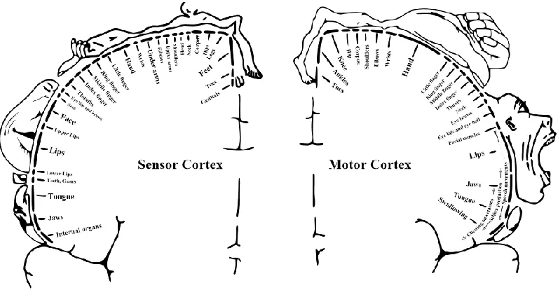
Figure 7: Homunculus model of the sensorimotor cortex, showing the layout of different body parts ... 18

Figure 8: a) Event-driven discrete control, based on transient neurological phenomena, such as movement-related potentials or P300; the return to the NC state is automatically done by the brain. b) State-driven discrete control: the user has the ability to initiate, maintain and release an intentional control state. Adapted from the technical report on self-paced BCI by Mason et al [8] ... 24

Figure 9: Event-driven BCIs allow only transitions between each IC state and NC, while state-driven BCIs allow all possible transitions ... 24

Figure 10: Depending on the distribution of IC and NC states in feature space, a single linear classifier might not be able to separate the two IC states from NC, if both IC states are considered one class ... 29

Figure 11: Electrode layout for dataset 1 of BCI Competition IV... 32

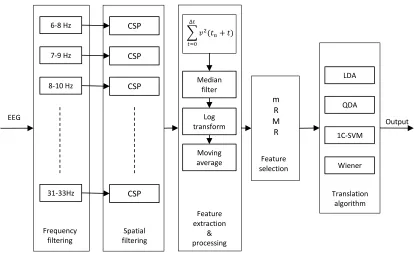
Figure 12: Block diagram of the BCI architecture ... 33

Figure 13: The CSP algorithm finds a set of virtual channels which maximize variance differences between two classes ... 34

Figure 14: Processing steps of our feature vectors ... 35

Figure 15: Two-stage detection and classification of IC states ... 38

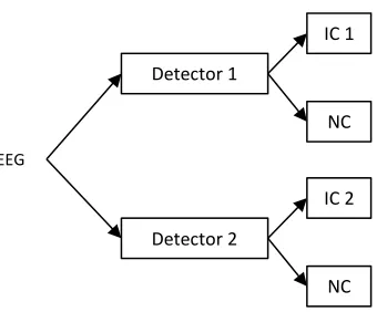
Figure 16: Separate detection of each IC state ... 39

Figure 17: Direct three-state classification ... 39

Figure 18: SVMs determine the hyperplane which maximizes the distance to the nearest training points ... 42

Figure 19: Finite impulse response topology of order M ... 43

Figure 20: The patterns of the three most relevant spatial filters for IC/NC discrimination extracted for each subject and the corresponding frequency bands ... 46

Figure 21: Mutual information between extracted features and the desired output for IC/NC discrimination with respect to the number of features ... 47

Figure 22: Mutual information between extracted features and desired output for IC/NC discrimination with respect to the window position within the trial ... 48

(6)

2

Figure 24: Mutual information between extracted features and the desired output for IC discrimination with

respect to the number of features ... 50

Figure 25: Mutual information between extracted features and desired output for IC discrimination with respect to the window position within the trial ... 51

Figure 26: LDA, QDA and one-class SVM detection rates in differential mode. Error bars represent the percentage of misclassified, yet detected IC states. TPi represents the true positive rate of IC state i, TP is the average true positive rate of IC detection. All TP rates correspond to an FP rate of 1% or lower. ... 53

Figure 27: LDA, QDA and one-class SVM detection rates in parallel mode. Error bars represent the percentage of misclassified, yet detected IC states. TPi represents the true positive rate of IC state i, TP is the average true positive rate of IC detection. All TP rates correspond to an FP rate of 1% or lower. ... 54

Figure 28: LDA and QDA detection rates for direct 3-state classification. Error bars represent the percentage of misclassified, yet detected IC states. TPi represents the true positive rate of IC state i, TP is the average true positive rate of IC detection. All TP rates correspond to an FP rate of 1% or lower. ... 55

Figure 29: Average IC detection rates for all subjects and classifier designs, and their standard deviation between subjects. Subscripts 1C, D, P and 3C represent one class (IC/NC), differential, parallel and direct 3-state classification, respectively ... 56

Figure 30: Influence of different parameters on detection rate. First column: classifier trained with average sample values, log transformed; second column: classifier trained with all samples from the window, log transformed; third column: all samples, no log. A window size of one sample is equivalent to not performing the respective operation. All TP rates correspond to an FP rate of 1% or lower. ... 58

Figure 31: Influence of smoothing operations on hold time... 60

Figure 32: TP rates for FP rates ranging between 1% and 10% ... 61

Figure 33: Relative improvement in TPR due to the use of refractory periods at two FPR values ... 63

Figure 34: Influence of the selection intervals on TP rate. Four sizes and four offsets are tested, of 0.5, 1, 1.5 and 2 seconds. For each combination, the best dwell and refractory periods are found. On the axis they are grouped with respect to the size, hence there are four groups [(size1,offset1), (size1,offset2)…], [(size2,offset1),(size2,offset2)…] etc. The ticks represent the size of the selection window, thus the tick following that at 1.5s corresponds to a size of 1.5s and an offset of 1s, thus a 1.5s window centered at 1.75s 65 Figure 35: Comparison between three approaches in cross-validation (CV) and evaluation (Eval). Values are averaged over all subjects and shown with the standard deviation. The default configuration uses the one second selection interval found in feature selection and no refractory period; +refractory adds the use of refractory period; +optimized selection uses both optimal training intervals and refractory periods. ... 66

Figure 36: Event analysis for LDA on the evaluation data, with TP rates as a function of event duration. Refractory periods and the optimal training intervals are used. The TPR above each plot is the TP rate of the corresponding IC state, averaged over all event durations. FPR is the sample FP rate, FPRE is the event FP rate ... 68

Figure 37: Inter-FA periods distribution for LDA. The minimum and maximum time between false activations is given above each plot. ... 69

Figure 38: Influence of the feature processing pipeline in terms of detection rate, mean squared error and mutual information, averaged over all subjects. ... 70

Figure 39: Detection rates for the Wiener filter (left) and comparison to LDA (right). Error bars represent the percentage of misclassified, yet detected IC states. TPi represents the true positive rate of IC state i, TP is the average true positive rate of IC detection. All TP rates correspond to an FP rate of 1% or lower. ... 71

Figure 40: Influence of tap delays on TP rate, event FP rate and response time. One tap delay is equivalent of using 100 ms of past data. The shaded area in the response time plots represents the standard deviation... 74

Figure 41: TP rates of the Wiener filter for FP rates ranging between 1% and 10% ... 75

Figure 42: Regression results on the evaluation data, with the original targets (Orig), with the ones determined by the genetic algorithm (+GA), and the additional use of refractory periods (+RP). ... 77

(7)

3

Figure 44: Inter-FA periods distribution for the Wiener filter. The minimum and maximum time between false activations is given above each plot. ... 79 Figure 45: True positive rates and event false positive rates of linearly combining classifier outputs with a genetic algorithm. Results are averaged over all subjects and shown with the standard deviation. On the x

(8)

4

List of tables

Table 1: The number of spatial filters selected for each subject, class and frequency band for NC/IC discrimination... 45 Table 2: The number of spatial filters selected for each subject, class and frequency band for IC discrimination... 48 Table 3: TP rates of IC detection for different classifiers at 1% FP rate. Both IC states are treated as one class ... 52 Table 4: Influence of dwell time and refractory period on TP rates for a maximum FP rate of 1%. The left part of the table shows the original TP rates obtained with no dwell or refractory post-processing. The right part of the table shows the TP rates obtained with the optimal dwell and refractory periods. FPROrig is the initial FP rate obtained at the corresponding TP rates, FPROptim is the FP rate after post-processing. Numerical subscripts of TP rates indicate the IC state, Avg indicates their average. ... 62 Table 5: Influence of dwell time and refractory period on TP rates for a maximum FP rate of 1.5%. For a detailed description refer to the caption of Table 4. ... 62 Table 6: Average true positive rates with the original labels and with the ones determined by LDA. The target values are expressed in terms of their mean and standard deviation ... 72 Table 7: Average true positive rates with the original labels and with the ones determined by the genetic algorithm ... 72 Table 8: Influence of dwell time and refractory period on TP rates of the Wiener filter for a maximum FP rate of 1%. The left part of the table shows the original TP rates obtained with no dwell or refractory post-processing. The right part of the table shows the TP rates obtained with the optimal dwell and refractory periods. FPROrig is the initial FP rate obtained at the corresponding TP rates, FPROptim is the FP rate after post-processing. Numerical subscripts of TP rates indicate the IC state, Avg indicates their average. ... 76 Table 9: Ratios of sample and event FP rates in cross-validation (CV) and on the test set, respectively. RP

(9)

5

List of acronyms

1-NN 1-Nearest Neighbour

ALS Amyotrophic Lateral Sclerosis AUC Area Under (ROC) Curve BCI Brain-Computer Interface BMI Brain-Machine Interface BOLD Blood Oxygen Level Dependent CNS Central Nervous System CSF Cerebrospinal Fluid CSP Common Spatial Patterns DBI Direct-Brain Interface

DSLVQ Distinction Sensitive Learning Vector Quantization DWT Discrete Wavelet Transform

ECoG Electrocorticography EEG Electroencephalography

EMG Electromyography

EOG Electrooculography

ERD Event-Related Desynchronization ERP Event-Related Potential

ERS Event-Related Synchronization FLD Fisher Linear Discriminant FIR Finite Impulse Response FPR False Positive Rate GMM Gaussian Mixture Model IC Intentional Control ITR Information Transfer Rate LDA Linear Discriminant Analysis

LF-ASD Low-Frequency Asynchronous Switch Design LFP Local Field Potential

ME Motor Execution

MEG Magnetoencephalography

MI Motor Imagery

MRP Movement-Related Potential

MSE Mean Squared Error

NC No-Control

PSD Power Spectral Density

QDA Quadratic Discriminant Analysis ROC Receiver Operating Characteristics SCP Slow Cortical Potential

SMR Sensorimotor Rhythm

SNR Signal-to-Noise Ratio

SQUID Superconducting Quantum Interference Device SSVEP Steady-State Visually Evoked Potential SVM Support Vector Machine

TF True-False Difference TPR True Positive Rate

(10)

6

Introduction

Humanity has always been fascinated by the possibility of interacting with the outside world only through the power of the mind. Throughout history, the apparently unlimited potential of the human brain has often led philosophers and scientists on a path of trying to prove that there is more to the mind than what we know. A fine example are the pioneering studies of Hans Berger in the late 20’s, which have led to the development of electroencephalography (EEG) and ultimately paved the way for modern neuroscience, and were motivated by his quest to find proof of telepathic

abilities in humans [1].

Nowadays, the blazing advances in diverse fields such as medicine, physics and engineering have allowed scientists to gain a much deeper understanding of the brain’s inner workings, and the exponential progress of technology promises to bring such developments to the masses, ultimately for the goal of an increased quality of life. A promising and relatively new direction is the field of brain-computer interfaces (BCI), which seeks to give people the capability of controlling various devices through the electrical activity of the brain.

As BCI technology steadily moves out of the lab and into hospitals, homes, and even military use, one pressing issue still remains. Due to the high complexity and apparent randomness of our brain, it is not very clear how to distinguish intentional commands from the seemingly stochastic ongoing cerebral activity. The problem of self-paced operation for BCI attracted the interest of many researchers in the past decade, but a widely accepted solution has yet to be found.

Motivation and objectives

Throughout the literature, one can find several studies related to self-paced BCI, each with different subjects, methods and experimental protocols. Deciding on a specific methodology is thus rather difficult, as the results of these studies cannot be directly compared because of the large variability between them. Differences in experimental protocol, subjects’ experience with BCI and reported performance metrics all hinder the process of making educated decisions on the many possibilities in designing self-paced BCIs.

What therefore seemed to be lacking was a comparative review of the different approaches to the problem, and this is exactly the gap that this thesis attempts to fill. By no means however do we claim that it is a complete overview of all possible methods and their combinations, simply because of the huge number of possibilities.

(11)

7

The first research question we address concerns the choice of an appropriate translation algorithm. Not only different machine learning methods, but also different implementation schemes are possible for classification in a self-paced context. One could opt for a two-stage design, in which the first classifier would detect intentional control (IC) commands of any kind, and the second would assign them to one of the possible classes. This seems to be the most popular choice in self-paced BCI research, but it is not the only one. A single classifier could be trained to directly distinguish between no control (NC) and the possible IC states. A third option is to train one classifier for each IC state, and to the best of our knowledge this approach has not even been tested in previous research. We hypothesize that the common approach of considering multiple IC states as one class is highly inappropriate, mainly because the neurophysiological phenomena underlying different IC states are chosen to be as different as possible.

To decrease incorrect activations of self-paced BCIs, specific tools are used, such as the refractory period or the dwell time. The second research question is how large and reliable is the performance gain obtained with such methods. To this end, appropriate evaluation criteria need to be defined. A wide variety of performance metrics exist for the evaluation of self-paced BCIs, yet no consensus exists regarding which is most informative. It is possible that a truly informative description of performance could not even be obtained by using a single metric. The third research question aims to find which evaluation criteria are most important for self-paced BCIs.

In the hope of objective, reproducible and more meaningful results, the methods under analysis are applied on a publicly available dataset, specifically designed for the evaluation of self-paced BCIs.

Report outline

(12)

8

Chapter I

Introduction to BCI

1 Objective of BCI research

Brain-computer interfaces, also called brain-machine interfaces (BMI) or direct brain interfaces (DBI), are a direct communication pathway between the brain and a computer or some other external device. BCIs convert electrophysiological signals of the central nervous system (CNS) into meaningful messages and commands that act on the outside world and accomplish the user’s intent, much in the same manner as conventional neuromuscular pathways. In that sense, a BCI replaces nerves and muscles with hardware and software that measure brain activity and

translate it into actions [2].

Assistive technology

Presently, the first and foremost objective of BCI research is restoring mobility and/or communication to those that have lost these abilities. Several neuromuscular disorders, such as amyotrophic lateral sclerosis (ALS), stroke, brain and spinal cord injuries, muscle dystrophies and many more affect millions of people worldwide and impair neural pathways or the muscles themselves. In extreme cases, patients might lose all muscle control, including eye movements and

respiration, leaving them completely locked-in to their bodies with no ability of communication [2].

In such cases, restoration of even basic communication abilities would increase the patients’ quality

of life and independence, as well as reducing social isolation and the cost of care [3]. The most

desired outcome of assistive BCIs would be the reanimation of a paralyzed limb [4] but short of that

brain-controlled robotic prostheses are also highly desirable.

Augmentative technology

The new control possibilities offered by BCI could also be valuable for healthy users, enriching their experience in various games or applications. At the present moment however, BCIs do not bring any benefit to healthy users, except for the possible joy of using a novel technology and a more immersive experience in some contexts. Presently, it can be argued that the only BCIs that healthy users might consider are EEG-based, as they are non-invasive and relatively cheap.

However, considering the modest information transfer rates (ITR) of current EEG-based BCIs1 (25

– 35 bits per minute [6]), it is hard to see a reason why present-day healthy users would choose a

slow, cumbersome and error-prone control input over the traditional mouse and keyboard input. This is not to say that we do not have faith in the future success of BCI; one must admit that the relative success of a technology partly depends on its availability to the masses. Even with the spectacular progress of BCI research in the past decades, it is no doubt that its most influential breakthroughs and applications are still to come with widespread adoption of the technology by healthy users.

1

(13)

9

2 Structure of a BCI system

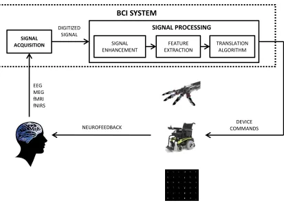
Throughout the literature there are several functional models of BCIs presented but considering the variability of different implementations they can be reduced to five basic components: signal acquisition, signal enhancement, feature extraction, the translation algorithm and feedback. A schematic model based on these components is presented in Figure 1. For a more

[image:13.612.123.536.198.494.2]

detailed functional model of BCI the reader is referred to the work of Birch and Mason [7, 8].

Figure 1: Functional model of a BCI system

Signal acquisition

Signal acquisition is the process of recording brain activity over time. Cortical activity can be inferred by measuring the electrical, magnetic or metabolic responses of the brain, through various techniques which will be discussed shortly.

Signal enhancement

Signal enhancement refers to techniques used to increase the signal-to-noise ratio (SNR) or reduce dimensionality. Undesired components of the signal, called artifacts, which are not a result of brain activity, are also removed in this step. These may include the 50/60 Hz power-line noise, various electromagnetic interferences and artifacts resulting from physical movements or hardware faults. Artifact detection and correction is a highly specialized and complex field in itself. It often requires additional sensors and measurements, such as recording eye movements through

EEG MEG fMRI fNIRS

DIGITIZED SIGNAL

SIGNAL

ACQUISITION FEATURE

EXTRACTION

TRANSLATION ALGORITHM SIGNAL PROCESSING

BCI SYSTEM

DEVICE COMMANDS NEUROFEEDBACK

(14)

10

electrooculography (EOG) or muscle activity through electromyography (EMG). Some applications skip this process altogether as possible artifacts might not influence the frequency bands of interest.

Feature extraction

The process of feature extraction transforms the measured cortical activity into meaningful and useful representations for predicting the intent of the user. In many cases feature extraction involves transforming the signal to a different domain and calculating relevant characteristics based on a priori knowledge of the neurological phenomena under analysis.

Translation algorithm

The translation algorithm of a BCI system converts the extracted features into a discrete or continuous control signal that is an estimation of the intent or mental state of the user (within the analyzed possibilities, of course – BCIs don’t read minds). BCI spellers in which users select letters on the screen is an example of discrete output, while applications in neuroprosthetics require real-valued output for controlling each joint of the artificial limb.

Feedback

The final step is to provide the user with information on the BCI predictions. This usually consists of displaying the result on a computer screen or issuing the associated command to a device, such as an actuated wheelchair or prosthetic limb. Feedback is very important in real-world applications, as the brain is capable of reorganizing neural connections for the purpose of learning and adaptation. This phenomenon is known as neuroplasticity and, in essence, is no different than learning to walk or to speak at an early age.

3 Recording techniques

There are quite a few methods available for recording cortical activity, each with specific strengths and weaknesses. While the brain is essentially an electrical machine, neuroimaging techniques have been developed that are also sensitive to its magnetic and metabolic activity. Following is a brief description of each technique.

3.1 Invasive methods

As the name suggests, invasive neuroimaging techniques require surgery for the implant of electrodes which measure the electrical activity of single neurons or neural ensembles. Given the close proximity to the grey matter, these methods currently offer the best quality signals and consequently the most natural control possibilities of prosthetic limbs. They are divided in two categories, depending on whether electrodes are implanted inside brain tissue or on the surface of the cortex.

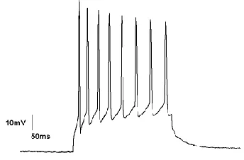
3.1.1 Intracortical electrodes

The most invasive type of neural implant consists of microelectrode arrays usually

(15)

11

[image:15.612.253.425.187.300.2]

activity of a single neuron can be measured. The activation of a neuron produces a so called action potential, which is the most basic form of neural activity and manifests as a sharp increase in the electric potential of a neuron’s membrane, typically from -70 mV to several tens of millivolts. Neurons can fire up to 100 times per second and the resulting sequence of voltage impulses is called a spike train (see Figure 2), which forms the basis of information processing within the brain and can be captured by intracortical electrodes.

Figure 2: Sequential action potentials form spike trains

The firing patterns of multiple neurons can synchronize and the summation of their synaptic currents produces oscillations in the electric potential of local extracellular space. These oscillations are called local field potentials (LFP) and can also be captured by intracortical implants. These electrodes therefore capture either the firing rates of single neurons or local field potentials of several neurons and translate them into complex movements.

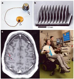
After extensive training of monkeys in a reaching and grasping task, it was shown that the firing patterns of only 32 neurons are sufficient to perform the same movement directly with a

robotic limb [10]. In 2004, Donoghue’s group presented a highly successful demonstration of an

invasive BCI [11], in which a tetraplegic subject could successfully check e-mails, control the TV,

(16)

12

Figure 3: a) The BrainGate sensor resting on a US penny and the percutaneous pedestal which connects the sensor to the rest of the system. b) Close-up of the 10 × 10 microelectrode array. c) Location of the sensor. d) The first participant in the BrainGate trials. Picture taken from the original article published

in Nature [11]

3.1.2 Electrocorticography (ECoG)

A less invasive option is electrocorticography, which consists of electrode arrays placed directly on the surface of the cortex. The signals thus recorded are a mixture of several LFPs, smeared and attenuated by the layers of brain tissue and cerebrospinal fluid (CSF). Because ECoG implants are only used by neurosurgeons for the purpose of clinical monitoring and localization of seizure foci in epileptic patients, the number of human subjects for ECoG research is rather

limited [12]. Nevertheless, ECoG signals were successfully used for decoding two-dimensional

hand movements with an accuracy comparable to what is achieved in monkeys with intracortical

microelectrodes [13]. In an ECoG study on monkeys, Chao et al proved that ECoG signals can be

used for decoding self-paced three-dimensional arm movements, again with comparable performance to that obtained by more invasive techniques. Another highly promising result of this study was that predictive performance remained stable across several months with no need for

[image:16.612.190.493.72.395.2]

(17)

13

3.2 Non-invasive methods

Invasive BCIs are clearly well suited for restoring mobility and communication to those in need, but they also pose the risks normally associated with brain surgery, such as infection and

tissue damage [15]. Even so, it is conceivable that patients suffering from severe neuromuscular

disorders such as amyotrophic lateral sclerosis, stroke or spinal cord injuries might choose the invasive option if there is no alternative. This would not be an option for healthy users however. Fortunately, the majority of BCI research focuses on non-invasive methods and continued technological advancements in both hardware and software hold promise for the future of such techniques.

3.2.1 Electroencephalography (EEG)

EEG is the oldest technique for measuring brain activity. It was developed by Hans Berger

in 1929 [1] and almost 90 years later it continues to be a valuable tool in both clinical and research

applications. EEG measures brain activity through sensitive electrodes placed on the scalp of the subject. The number of electrodes varies depending on the application and montages of up to 512 electrodes are used. Electrolytic gel is usually applied to form a conductive bridge between skin and electrode for decreasing impedance and the recorded voltages are amplified with a factor commonly

ranging between 103 and 105. EEG amplitudes are quite weak, in the order of microvolts, and the

recorded activity is a spatial integration of multiple local field potentials. Thus, the spatial

resolution of EEG is quite poor (~ 1 cm [16]) but source localization methods can be used in

multi-channel recordings for improving resolution. Furthermore, EEG is susceptible to movement artifacts, electromagnetic interference, muscle activity, and the signal is severely degraded because of the meninges, cerebrospinal fluid (CSF) and the skull.

One advantage of EEG is considered to be the high temporal resolution, as sampling rates of 4 KHz or higher are quite common in such devices. However, the usefulness of such a high sampling rate is limited due to the 1/f nature of EEG spectra (see Figure 4). As the amplitude of

oscillations is proportional to the number of synchronously active neurons [17], slowly oscillating

cell assemblies comprise more neurons than fast oscillating ones [18]. The signal to noise ratio of

EEG is rather poor to begin with, and the severe degradation of high frequencies drastically limits the usefulness of high sampling rates.

(18)

14

Figure 4: Typical EEG power density spectrum (left) and close-up of the low-frequency range (right) depicting the 1/f nature of EEG spectra. Notice the 50 Hz power line noise and its harmonics (left) and

the peaks close to 10 and 20 Hz (right) corresponding to alpha and beta rhythms, respectively

3.2.2 Magnetoencephalography (MEG)

Electrical currents flowing through the axons of neurons induce a very weak orthogonal magnetic field, which can be measured outside the skull by means of magnetoencephalography. Unlike the electric field measured by EEG, the magnetic field is barely influenced by the surrounding brain tissue, CSF and skull. Furthermore, MEG has a spatial resolution of

approximately 5 mm [16], superior to that of EEG [19], and also has a wider frequency range [20].

BCI experiments with MEG in two-dimensional control provided satisfactory results, achieving

69% accuracy in a four-class scenario [21].

MEG-based BCIs are still far away from widespread use. The magnetic field produced by

the brain is very weak, roughly 10 fT (10-14T), many orders of magnitude weaker than the Earth’s

magnetic field, which is about 0.5 mT. MEG therefore requires magnetically-shielded rooms. MEG devices are also bulky and expensive, as they consist of arrays of extremely sensitive SQUID (superconducting quantum interference device) detectors which need to be cooled in liquid helium (see Figure 5). Furthermore, while EEG recordings permit some level of head movements, MEG requires complete stillness.

0 10 20 30 40 0

10 20 30 40 50 60

Frequency [Hz]

P

o

w

e

r/

fr

e

q

u

e

n

c

y

[

d

B

/H

z

]

0 100 200 300 400 500 -50

-30 -10 10 30 50

Frequency [Hz]

P

o

w

e

r/

fr

e

q

u

e

n

c

y

[

d

B

/H

z

(19)

15

Figure 5: Participant in an MEG study at the National Institute of Mental Health, USA

3.2.3 Functional magnetic resonance imaging (fMRI)

Up to this point, we have discussed neuroimaging techniques that record brain activity based directly on electromagnetic measurements. A different approach is to indirectly infer cortical activity by measuring the metabolic response of specific brain regions, particularly the blood oxygen level dependent (BOLD) response. Active neurons produce an increase in oxygen-rich blood flow in surrounding tissue, and this change can be captured by functional magnetic resonance imaging. The prefix “functional” refers to the usage of standard MRI techniques for the imaging of blood flow instead of structural tissue.

fMRI provides good spatial resolution (1 mm [16]) and was successfully used for online

two-dimensional control of a robotic arm by a human subject [22]. Its practical use in BCI is

however limited by the large, expensive equipment and the rather poor temporal resolution of BOLD signals (up to several seconds), as the hemodynamic response is slower than the underlying neural activity.

3.2.4 Functional near-infrared spectroscopy (fNIRS)

(20)

16

performance in BCI applications is lower than what can be achieved by EEG [23] and they also

suffer from the relatively high latency of the hemodynamic response.

3.3 Conclusion

While in clinical and neuroscience research applications expensive and non-portable equipment have their use, for practical, everyday BCIs, portability is a must. Leaving invasive methods aside for similar reasons, we are thus left with a choice between EEG and fNIRS.

Combining the two techniques might prove to be most beneficial. A recent study by Fazli et al found a 5% increase in classification accuracy in a two-class motor imagery experiment by complementing EEG with fNIRS. The increase is modest though, and EEG surpassed fNIRS in accuracy for both executed and imaginary movements. An interesting detail is that while EEG performance dropped 13% (from 90.8% to 78.2%) in the case of motor imagery (MI) compared to motor execution (ME), fNIRS performance remained quite stable, and quite surprisingly the oxygenated hemoglobin feature even had a slightly higher classification accuracy (71.7% for MI

compared to 71.1% for ME) [24].

Simultaneous recordings of EEG and fNIRS will most likely be a hot BCI research topic in the years to come, but the slow BOLD response will still hamper the information transfer rates achievable by fNIRS systems. Berger would be proud to know that even though we landed a man on the Moon and have supercomputers in our pockets, his invention still holds the most promise for the future of BCI. The rest of this paper will be therefore focused on EEG-based BCIs.

4 Neurological phenomena

A common myth surrounding BCIs is that they read minds. While we hope that the above review of neuroimaging techniques shed some light on the difficulty of capturing brain activity, we must stress that BCIs (especially non-invasive variants) simply rely on the detection of specific cerebral patterns and associate them with commands that can be outputted to external devices. These patterns can be either a result of the subject performing some mental task or a natural response of the brain to some stimulus. Neurological phenomena generated as the result of

cognitive processes are called endogenous, while the ones evoked by an external stimulus are called

exogenous.

To gain a better understanding of the inner workings of BCI systems, in this section we will outline the most important neurological phenomena that are presently used in EEG-based BCIs.

4.1 Sensorimotor rhythms

(21)

[image:21.612.145.508.71.324.2]

17

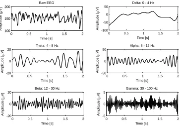
Figure 6: Typical brainwaves and their associated frequency bands. Notice the inverse relation between amplitude and frequency

In addition to the rhythms illustrated above, a particularly important brainwave for BCI is the mu rhythm, which commonly occupies a similar frequency band as alpha (8 – 13 Hz), but has a distinct arc shape and is predominantly found over the sensorimotor cortex. The mu and beta rhythms are the most important to BCI as their amplitudes are modulated by real or imaginary movements. These modulations have distinct topographical distributions for different body parts.

All muscles and organs are innervated by neurons, the wiring of our body responsible for carrying information. Muscular commands are downloaded from the brain and sensory information is uploaded back. The cortical areas devoted to controlling or feeling different body parts have distinct locations on the sensorimotor cortex. Neuronal networks responsible for adjacent parts of the body are also located next to one another, but their area is not a reflection of the physical size of the body region they control, but rather of the number of neurons that innervate the respective region. The representation of the body within the brain is often called the cortical homunculus and is illustrated in Figure 7.

0 0.5 1 1.5 2

100 150 200 Time [s] A m p lit u d e [ V] Raw EEG

0 0.5 1 1.5 2

-100 -50 0 50 Time [s] A m p lit u d e [ V]

Delta: 0 - 4 Hz

0 0.5 1 1.5 2

-20 0 20 Time [s] A m p lit u d e [ V]

Theta: 4 - 8 Hz

0 0.5 1 1.5 2

Alpha: 8 - 12 Hz

0 0.5 1 1.5 2

Beta: 12 - 30 Hz

0 0.5 1 1.5 2

(22)

[image:22.612.127.525.84.301.2]

18

Figure 7: Homunculus model of the sensorimotor cortex, showing the layout of different body parts

Certain events can synchronize or desynchronize distinct neuronal networks, resulting in frequency and spatially specific increases or decreases in amplitude. Similar to ERPs, these changes are time-locked to the event, but are not phase-locked, thus cannot be extracted by time-domain

averaging, but rather by spectral analysis [25]. An increase in band power is called event-related

synchronization (ERS) and correspondingly, a decrease is referred to as event-related desynchronization (ERD).

Idling periods are characterized by synchronous neural firing and generally large power in the mu and beta bands. Executed, imagined, or attempted movements (in the case of paralyzed patients) desynchronize neural activity, producing ERD of the mu and beta rhythms. Upon completion of the movement, an increase in power called post-movement ERS is usually found,

especially in the beta band [25]. The distinct topographical mapping means that movements of

different body parts will elicit power modulations in specific brain regions, thus forming the basis of sensorimotor-based BCIs.

These BCIs have many advantages. Paradigms requiring the user to change gaze direction for selecting a letter do not rely solely on brain activity, as they also require ocular movements.

They are therefore called dependent BCIs [2]. SMR-based BCIs do not rely on any stimulus or

muscular output path, but rather on internally generated events, such as an imaginary or attempted

movement, thus being independent BCIs which could be used even if the senses are impaired. This

is also true for SCP-based BCIs, but the SMR paradigm is less affected by EOG artifacts, thus potentially requiring fewer sensors and processing power invested in artifact correction.

Furthermore, SMR systems are a valuable tool in rehabilitation [26] and in potential

neuroprosthetic applications due to the movement-related paradigm. In what can be considered state-of-the-art in EEG-BCI, Wolpaw et al have demonstrated for the first time 3D cursor control,

potentially validating EEG as a source of control for artificial limbs [27]. The study shows that the

(23)

19

control became easier with training as the precise nature of the mental task became less important and control became more automatic. This is similar to the training of regular motor skills, such as walking. The authors also compare the 2D target acquisition time for the intracortical BrainGate

implant [11] with a previous motor imagery EEG study [28] and show that surprisingly, EEG

control had the same success rate and latency as intracortical implants.

4.2 Evoked potentials

An evoked potential is the brain’s response to an external sensory stimulus. In EEG recordings, evoked potentials manifest as slow changes in voltage. The most commonly used evoked potentials in BCI are visually evoked potentials. Flickering light at a given frequency elicits cortical activity at the same frequency in the occipital lobe, which governs visual information processing. This particular type of evoked potential is called the steady-state visually evoked potential (SSVEP). Thus, when two or more targets are used, each with a different frequency, the user’s gaze direction can be inferred. This paradigm can be used for communication and control in BCI systems. As a matter of fact, the first BCI developed by Vidal in 1973, used SSVEP for

navigating a maze [29]. The pioneering work of Jacques Vidal was the first proof on the feasibility

of EEG-based communication and also introduced the term “brain-computer interface”.

4.3 Event-related potentials

A particular type of evoked potentials is the event-related potentials (ERP), which are the result of higher-level processes, involving attention, expectation or memory, among others. The most common ERP employed in BCI research is the P300 response, which manifests as a positive voltage deflection appearing roughly 300 ms after the presentation of a particularly important visual, auditory or somatosensory stimulus, when interspersed with other frequent or routine

stimuli [2]. The most common application of P300 is in speller devices, where the user is presented

with a 6 × 6 matrix of letters, numbers and/or commands. Each column and row is flashed multiple times for averaging EEG noise, and the P300 is detected only for the column or row which contains

the desired symbol. Thus, the user’s intended choice can be inferred [30]. As with SSVEP, one

advantage of P300 is that it is a natural response of the brain, thus requiring no user training.

4.4 Slow cortical potentials

Unlike evoked potentials, slow cortical potentials (SCP) are not dependent on external stimuli, but rather reflect an increase or decrease in cortical activity. They are among the lowest frequency features detectable by EEG, and manifest as negative or positive voltage deflections over the course of 0.5 – 10 seconds. Negative SCPs are associated with movement, while positive ones

are commonly associated with reduced cortical activation [31]. With extensive user feedback

training, up to several months, people can learn to control the polarity of SCPs. This self-regulation can be used for binary selections in BCIs, and formed the basis of the “Thought Translation

Device” BCI, used to restore basic communication abilities in ALS patients [32]. Besides the

obvious drawback of requiring prolonged user training, SCP-based BCIs provide relatively slow

communication speeds, at a rate of 0.15 – 3 letters per minute [2], and due to their low frequency

(24)

20

4.5 Conclusion

The obvious advantage of BCIs that use exogenous neurological phenomena is that they require no user training. The downside of such systems is the constant commitment of a sensory

modality such as vision [33] to potentially repetitive stimuli that might cause user fatigue and

frustration. Endogenous neurological phenomena indeed require some level of user training for generating stable and consistent cortical patterns, but once the user familiarizes with the control method, it is expected that control will gradually become easier and more natural. Furthermore, because such independent BCIs do not rely on any sensory pathways, they are highly valuable for patients with impaired senses. It comes to no surprise that more than 80% of BCI research is

(25)

21

Chapter II

The self-paced BCI

We have seen that, when presented with specific stimuli or performing certain mental tasks, characteristic changes affect cerebral activity. These cortical patterns can be used for communication and control in brain-computer interfaces. Most recording techniques are noisy and spontaneous EEG activity in particular resembles a stochastic process with the relevant features for control buried in noise. This means that the characteristic patterns associated with possible output commands vary quite a lot and often overlap. Unlike traditional, deterministic communication systems in which noise mostly affects the transmitted message, in EEG-based communication noise is present all the time, whether the user desires to output a command or not. Until some complete model describing all possible EEG activity is established, we are forced to consider as noise all EEG activity except the characteristic neurophysiological phenomena used for control, depending on the paradigm. This can be troublesome, as the relevant EEG features are often smaller in amplitude than the noise itself; hence there is a considerable probability that spontaneous activity might emulate the control features without the user having intended to output a control signal.

This brings up an important topic: while in a discriminative scenario, such as distinguishing imaginary movements of the left and right hand, it is fairly easy to attain good performance

(>90%) [35], how do we go about distinguishing the active tasks from all other possible EEG

activity? To gain a better understanding of the problem, let us first put it better in context.

1 The no control (NC) state

In most communication systems and interfaces, self-paced control is not an issue. We pick up the telephone and call somebody if and when we want to, use computers when we desire and turn the steering wheel of a car only when needed. That is because such systems rely on physical interaction, and periods in which the user has no control (NC) intention are characterized by no input to the system. Such a clear delimitation is presently impossible to achieve with EEG-based BCIs, due to the spontaneous cortical activity that often resembles the one associated with periods of intentional control (IC).

NC support is necessary in all applications where frequent periods of intentional control are interspersed with periods of inaction. It is noteworthy to mention that the NC state is not the same as an idle or relaxed state in which the user tries to think of nothing, but rather entails these as sub-states. As discussed in section 4.1, these periods have distinct characteristics, such as large power in the mu band of sensorimotor rhythms, and represent only one possible type of NC. The NC state is therefore characterized by all possible cortical activities other than the ones used for intentional control. This tremendously complicates designs, as BCIs with NC support must handle the variety of additional tasks the user might be doing between IC periods, whether daydreaming or staring out the window for a few minutes, watching a movie for a few hours or performing any action other than trying to control the BCI. Arguably, it is unlikely that one can model all possible NC

(26)

22

One possibility would be to simply turn the BCI off when not needed. This could be performed manually by the user or through some automatic mechanism that would put the BCI into

a low-power state, similar to the “sleep” mode of laptops [8]. Implementing an automatic “sleep”

mode is not a solution though, as it implies that the system is already able to recognize long periods of inactivity, therefore entailing the availability of NC support. A solution for turning off the BCI is the so-called “brain switch”, a specific mental task that the user needs to perform in order to turn the BCI on or off. This has been experimented with mostly in hybrid BCIs, which use SSVEP for control and the post-movement ERS of brisk imagined foot movements as the brain switch. In such an experiment, the brain switch decreased false activations in NC periods from 5.4 to 1.4 per

minute [37]. However, the use of a brain switch does not resolve the intrinsic problem of NC

support for the primary BCI, and might not be convenient in many applications. For long periods of inactivity, turning the system off might indeed be beneficial and even necessary, but it is not an appropriate solution for the majority of everyday interactions which require short and frequent pauses, such as conversations or the navigation of a motorized wheelchair through the environment.

2 BCI control paradigms

For a better clarification of the problem, in the following we will review the various timing mechanisms used in BCI research and the different types of output. We adopt the classification

proposed by Mason et al in a technical report dedicated to self-paced BCIs [8].

2.1 Timing mechanisms

Synchronized control

In synchronized control, the BCI is periodically available to the user when it is on/awake and it does not support NC. The user is prompted via a cue when a control period (trial) starts and does not have the possibility of not issuing any command to the system. Especially for BCIs based on the modulation of sensorimotor rhythms, this is the predominant form of control and is also the most simple.

Constantly engaged

These BCIs are constantly available to the user but do not support NC. This is not a practical mode of control, as the user must continuously control the BCI and correct false activations during periods of inactivity. An example of such a system is the virtual keyboard speller developed by Scherer et al, a 3-class BCI in which users select letters with imaginary movements of

the left hand, right hand and foot [38].

System-paced

(27)

23

Self-paced

Self-paced control means that the BCI is constantly available to the user when it is on/awake and it supports NC. The user thus has full control over the BCI and uses it at his or her discretion. This is arguably the most natural form of control for any interface.

2.2 Continuous and discrete outputs

As discussed, BCIs can have either continuous or discrete outputs. The vast majority of classification procedures used in BCI gives a continuous output. An unknown sample goes through the same feature extraction and processing pipeline used in training and receives a score which represents its similarity to the known classes. This score can be either a distance measure (how close is the sample to each of the known classes in feature space) or a probabilistic one (what is the probability that the sample belongs to the known classes). Irrelevant of its nature, a discrete output can be obtained by simply applying a threshold on the continuous score.

Most BCIs which rely on exogenous neurological phenomena have discrete outputs, as to express the presence or absence of a certain stimulus. In general, presenting a measure of the similarity score is useful in endogenous BCIs for providing feedback, which in turn allows the user to learn and adapt. However, the desired type of output depends on the target application. For

example, in the case of the virtual keyboard developed by Scherer et al [38], the presented feedback

is continuous but the output is discrete, as the user chooses from a finite set of possible symbols. On the other hand, applications in neuroprosthetics might require continuous output for the precise control of each joint.

In general, self-paced applications benefit from continuous outputs, as the thresholding of similarity scores allows fine-tuning the balance between BCI sensitivity and false activations.

2.3 Event-driven and state-driven outputs

Mason et al describe two possible implementations of self-paced BCIs with discrete

outputs: event-driven and state-driven designs [8].

In event-driven self-paced BCIs, the user has the ability to initiate a state change whenever desired, but cannot maintain this state because of the transient nature of the underlying neurological phenomena. That is to say, the return to the NC state is automatically performed by the brain. Because of the automatic return to NC, event-driven designs lack the possibility of directly transitioning from one IC state to another IC state. BCIs based on movement-related potentials or P300 are common examples of event-driven designs.

(28)

24

Figure 8: a) Event-driven discrete control, based on transient neurological phenomena, such as movement-related potentials or P300; the return to the NC state is automatically done by the brain. b)

State-driven discrete control: the user has the ability to initiate, maintain and release an intentional control state. Adapted from the technical report on self-paced BCI by Mason et al [8]

While it may not become immediately apparent from Figure 8, the possibilities offered by state-driven BCIs are substantially larger, as the user has the option of maintaining an IC state or directly switching to another IC state. This is represented by the fully connected graph in Figure 9.

Figure 9: Event-driven BCIs allow only transitions between each IC state and NC, while state-driven BCIs allow all possible transitions

2.4 Conclusion

There is an important point to be emphasized here: self-paced control is an issue only for BCIs relying on endogenous neurological phenomena. Exogenous paradigms such as P300 or SSVEP are inherently self-paced, as the user pays attention to the stimulus only when desired. While false activations are still possible, they are less likely. So then why go through all the trouble of enabling self-paced operation for endogenous BCIs? Aside from the drawbacks already discussed in section 4.5, the requirement of an external stimulus makes P300 and SSVEP solutions rather unusable in one of the most sought-after BCI applications: the control of artificial limbs. In this context, endogenous BCIs are the only option, as they present another crucial advantage: they give the user the possibility to adapt and learn and ultimately better control the BCI.

ideal transducer

output N feature

space NC

ICA

initiate

A state

automatic release

duration of “on” time depends on classifier design feature

vector, f(t)

decision boundary

A

time

ideal transducer

output N feature

space NC

ICA

A

time decision boundary feature

vector, f(t)

initiate

A state

hold

A state

release

A state

NC IC 1 IC 2

(29)

25

Unsurprisingly, it becomes apparent that the very existence of such applications is conditioned on the availability of NC support.

Thus, from now on our discussion will be focused on endogenous neurological phenomena. State-driven BCIs based on sensorimotor rhythms seem the best candidate for self-paced operation, simply because they give the user full control over the transitions and durations of IC states.

3 Performance metrics for self-paced BCIs

Evaluating synchronized BCI experiments is not a challenge. For each trial, the true and predicted labels are known, thus a myriad of performance metrics can be derived. For a review,

interested readers are referred to the report of Schlögl et al [39]. One could argue that the same

holds true for self-paced BCIs as well. After all, we know the true label of each sample, thus we can compare it to the predicted label and apply the same evaluation criteria. The problem with this approach is that more often than not, self-paced data is unbalanced, i.e. there are many more samples from the NC state than from IC states. This means that many of the well-established criteria such as accuracy are no longer applicable. Consider a scenario where there are 9 times more NC samples than IC, and the system has 90% accuracy. Normally, such a performance would be considered very good, but it might very well be the case that the system classified all samples as NC, therefore achieving an accuracy of 90%. What is therefore needed are performance metrics that measure the detection rate of IC states (call them positives) and the rate of false detections during NC (call them negatives). Ideally, all IC states would be correctly detected and no false activations would occur during NC.

But this is only part of the story. While we can come up with adequate performance metrics for unbalanced data, we need to ask ourselves whether such “sample-by-sample” evaluations are actually meaningful. Consider the following scenario: there are 10 IC-related activations (call them events), each having 10 samples and we have two algorithms to evaluate. One algorithm correctly detects all 10 samples of only one out of the 10 events, while the other detects only one sample for each of the ten events. While neither of the two possibilities is exactly optimal, generally the second option is preferable. This type of evaluation is the most appropriate for self-paced BCIs and is called “event-by-event” evaluation.

3.1 Sample-by-sample evaluation

In sample-by-sample evaluation, each sample of the BCI output is compared to the label of the intended output for that sample. Different metrics can be used for this evaluation, such as the mean squared error, the mutual information between true and predicted labels, or the area under the ROC curve.

Mean squared error (MSE)

(30)

26

self-paced BCIs in the fourth international BCI competition2. What was most surprising about this

decision is that previously (in the third competition) the evaluation criterion for self-paced BCI was mutual information, which is generally considered to be a much better alternative.

In general though, the mean squared error is not a good indicator of performance for self-paced evaluations. Let us consider a three-state self-self-paced BCI with two IC states. Assuming the label of the NC state is 0 and the two IC states are represented by -1 and 1, misclassification errors between the two IC states will be larger than false activations, i.e. errors between 0 and ±1. While this might seem intuitive, we need to keep in mind that in most of the time the different IC states can be distinguished with satisfactory accuracy. The difficult part is distinguishing them from the NC state, and exactly this aspect is not emphasized by the mean squared error. The MSE is a highly informative metric in cursor control applications with continuous output, such as

neuroprosthetics [40], where the preciseness of control is to be evaluated.

Mutual information

The mutual information between two processes X and Y is a measure of the decrease in the

uncertainty of X when knowing Y, or vice versa. It is a symmetric function of their joint probability

distribution and is defined as:

( ) ∫ ∫ ( ) (_{( ) ( )} ( ) )

(1)

This is a highly desirable property of a BCI, as it is a direct measure of the user’s

intent [39]. For both discrete and continuous outputs, as well as different number of states, mutual

information is considered a relevant and informative performance metric. However, it is difficult to compare the results of different studies based on the mutual information, because this metric is also sensitive to the sample size of each state, which generally varies between studies.

Receiver operating characteristics (ROC)

The receiver operating characteristics (ROC) curve is a popular and insightful evaluation criterion for signal detection systems. It is created by varying the decision threshold of a binary classifier with continuous output and calculating for each step the true positive rate (TPR) and the false positive rate (FPR). The former is a measure of sensitivity, while the latter is a measure of specificity.

Considering that TP is the number of true positives (correctly classified positive samples),

P is the total number of positives, FP is the number of false positives (incorrectly classified

negative samples) and N is the total number of negatives, the true and false positive rates are given

by

(2)

2

(31)

27

These performance metrics are advantageous as they provide a natural solution to the issue of unbalanced data. The true and false positive rates can be combined in a single performance metric, the area under the ROC curve (AUC). The area under the ROC curve is equal to the probability that a random positive sample will be ranked higher than a random negative sample. An AUC of 0.5 represents random performance and an AUC of 0 or 1 represents perfect classification. While the AUC is only applicable in binary classification, multi-class extensions have been

proposed [41].

3.2 Event-by-event evaluation

The common practice in self-paced BCI evaluation is to report event-based TPR and

sample-based FPR [8, 36, 42]. The event-based TPR is defined as the number of successful

IC-related activations relative to the number of attempted IC states [8]. Therefore, it becomes

necessary to count multiple detections within a single event as a single true positive, otherwise multiple correct activations within an IC state can create the illusion of many successful detections,

when in fact only one event occurred [43]. A drawback of this approach for self-paced BCIs with

more than one IC state is the lack of a formal definition of classification errors between IC states. It is possible that more than one IC state is detected during an event, including the correct one. In this paper, such an event is counted as a true positive, but is considered a misclassification error between IC states.

Event-based false positive rates can be calculated as well, but this may lead to an overly pessimistic view on performance, as any false activation during an arbitrarily long NC period would label the whole non-event as a false positive. Because of the variable durations of NC states, sample-based FPRs are generally preferred. The standard practice is to report event-based TPR

corresponding to a sample-based FPR of 1% [36]. Fixing the FPR to a predefined value leaves only

one metric, the event-based TPR, which is more easily comparable between studies.

Another possibility of combining event TPR and sample FPR in a single metric is the

true-false difference (TF) introduced by Townsend et al [43] and defined as

(

) (3)

where E represents the number of IC events. In this context, all detections during a

non-event are counted as false positives, and a true positive is defined to be one or any number of detections during an event.

Detecting the no control state in self paced Brain Computer Interfaces