Solution of Singular Integrals in Mathematical Model of
Mode I Crack Near Strength Mismatched Interface
Sunil Bhat1, Vijay G. Ukadgaonker2
1School of Mechanical and Building Sciences, VIT University, Vellore, India 2Department of Mechanical Engineering, Indian Institute of Technology, Mumbai, India
Email: [email protected]
Received April 5,2012; revised May 2, 2012; accepted May 10,2012
ABSTRACT
Characteristics of Mode I crack near the interface of elasticity matched but plasticity and strength mismatched materials differ from those of the crack in a homogenous body. Interface body of different strength influences the plastic or cohe-sive zone at the crack tip in parent body. The mathematical model for load line opening of the crack near the interface in linear elastic regime involves singular integrals. The paper presents explicit solution of these integrals with the help of Cauchy’s principal value theorem. Cases of thin and thick welds between the materials are investigated. Solutions of the integrals are well substantiated. Final results are provided in a consolidated form.
Keywords: Crack Opening Displacement; Singular Integrals; Strength Mismatch; Weld Interface; Cauchy’s Principal
Value Theorem
1. Introduction
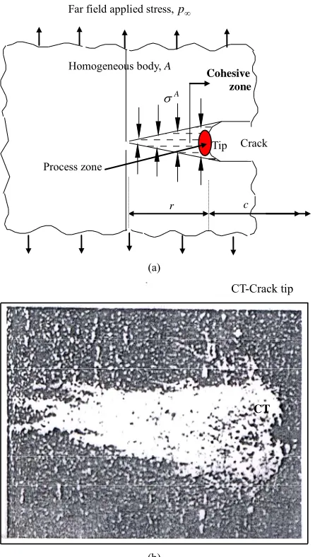
The material behaviour at the tip of the Mode I crack in a homogenous body is in general very complex and diffi-cult to describe by continuum mechanical models. The crack tip region where the material undergoes degrada-tion or damage is known as the process region. Refer
Figure 1(a). Micro-mechanical processes, viz. micro-
cracking in brittle materials and void initiation and coa-lescence in ductile materials create new traction free sur-faces or cracks in process region. Yielding occurs outside the process region. This zone is called as the plastic or cohesive zone. Cohesive zone is considered as the crack extension under the action of closing cohesive stress generated by elastic constraint exerted by surrounding non-yielded material over the cohesive zone. The cohe-sive stress is assumed equal to material yield strength in plane stress and 3 times the yield strength in plane strain conditions. Qualitative characteristics of the cohe-sive zone were experimentally verified by Hahn et al. [1].
They conducted experiments on cracked steel specimens and found the cohesive zone, as shown in Figure 1(b),
by etching the polished surface in front of the crack tip. In a bimaterial comprising elasticity identical but plas-ticity and strength mismatched constituents (like steels), the Mode I crack near the interface has the characteristics similar to the one in homogeneous parent body as long as the cohesive zone is in the parent body alone. The effect of approaching interface body of different strength is not
felt by the crack in such a stage because of similar elastic properties across the interface. But as the crack grows and reaches nearer to the interface, the increasing mag-nitude of crack tip stress field causes the cohesive zone to develop in the interface body. Consequently, the part of cohesive zone in the interface body is subjected to cohesive stress different from that acting over its portion in the parent body that triggers the effect of strength mis- match across the interface over the crack tip. The effect continues with increasing intensity as the cohesive zone spreads deeper into the interface body with crack growth and reaches the maximum when the crack tip touches the interface body with the cohesive zone fully in the inter- face body.
Cases of thin and thick welds between the steels are examined. Thin weld, obtained by non-fusion, solid state like friction welding between dissimilar steels leads to a single thin interface whereas a thick weld by fusion bonding from electron or laser beam welding results in two interfaces, one between the parent body and the weld and the other between the weld and the interface body. The parent body, the weld and the interface body have similar elastic properties but variable strengths of com-parable magnitudes.
2. Problem Definition
A
Cohesive zone
r c
Far field applied stress,p
Crack Tip Homogeneous body, A
Process zone
(a)
CT-Crack tip
CT
[image:2.595.314.536.70.476.2](b)
Figure 1. Crack tip cohesive zone and its experimental validation; (a) Crack tip cohesive zone; (b) Cohesive zone observed experimentally by Hahn et al. [1].
for this purpose in linear elastic regime.
2.1. Crack Near Thin Weld (Refer Figure 2) Half load line crack opening, v, in the cohesive zone of
size, r, in parent body A in stage I, Figure 2(a), subjected
to cohesive stress, A, under far field applied stress intensity parameter, , is of the following form [2]:
applied
K
02 1
d 2π
A r applied
K r
v
x E r x r x x
(1)
where, , is the modulus of elasticity of parent body, A. On integrating Equation (1), the expression for v,
as the function of distance x from the crack tip in the
cohesive zone is obtained as A
E E
At Tip
x = 0, y = 0 Far field applied stress,p
Interface body, B
Parent body, A
A
Thin weld
c r
Tip
Axis Crack
x,u Axis y,v
(a)
p
A
B
Crack
c a
l b
[image:2.595.63.286.84.478.2](b)
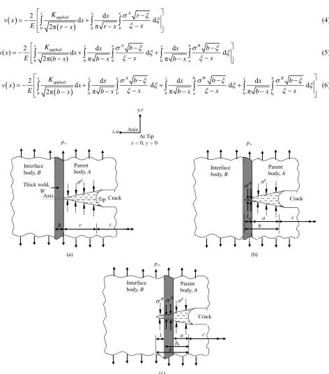
Figure 2. Stages of crack advancement towards a thin weld; (a) Stage I (Cohesive zone in parent body); (b) Stage II (Ex-tension of cohesive zone into interface body).
0 0 0
2 d
d d
π
2π
A
x x r
applied
K x r
v x x
E r x r x x
(2) Stage I is valid till the cohesive zone lies in the parent body i.e. the distance of the crack tip from the interface, a, fulfills the condition, ar.
Refer Figure2(b). The crack has grown ahead from
Stage I such that ar. The cohesive zone has
devel-oped in interface body, B, with its extent up to distance, l,
from the interface. Length of the cohesive zone, b, is
equal to (a + l). Since, , the following
ex-pression is written for v(x) in Stage II under simultaneous
action of different cohesive stresses
A B
E E E
A
and B in parent and interface bodies respectively with the help of
quation (2) E
applied
0 0 0 0
2 d d
d d
π π
2π
A B
x x a x b
a
K x b x b
v x x
E b x b x x b x
d x
(3)
2.2. Crack Near Thick Weld (Refer Figure 3) for v x
assume the following forms in Stages I, II and III in the case of thick weld:Using similar principles as in thin weld, the expressions
applied
0 0 0
2 dd
π
2π
A
x K x r r
x
v x x
E r x r x x
d
(4)
applied
0 0 0 0
2 d d
( ) d d d
2π( ) π π
A B
x x a x b
a
K x b x
v x x
E b x b x x b x
b
x
(5)
1
1
applied
0 0 0 0 0
2 d d d d d d
π π π
2π
b
A W B
x x a x x b
a b
K x b x b x
v x x
E b x b x x b x x b x x
d b
(6)
At Tip
x = 0, y = 0 x,u Axis
p
Interface body, B
Parent body, A
A
Crack
c
Tip Axis
Thick weld, W
y,v
r
p
Interface body, B
Parent body, A
A
Crack
c a
W
w l
b
(a) (b)
p
Parent body, A
A
Crack
c a
1
b
l
Interface body, B
B
W
b
[image:3.595.65.537.166.702.2](c)
Figure 3. Stages of crack advancement towards a thick weld; (a) Stage I (Cohesive zone in parent body); (b) Stage II (Spread
All the integrals, especially non-singular ones, in Equation (1) to Equation (6) need to be solved for ob-taining a usable form ofv(x).
3. Solution
Equations in important stages of crack growth towards the interface in bodies with thin and thick welds are solved as follows.
3.1. Crack Near Thin Weld In Stage II,
1 2 32
v x I I I
E
(7)where
applied 1
0
2
0 0
d , 2π
d
d , π
x
A
x a
K
I x
b x
b x
I
x
b x
and
3 0
d d
π
B
x b
a b x
I
x b x
Integral I1 is easily solved as
1 applied
2
π
I K bx
Integrals I2 and I3 are singular in nature and are
evalu-ated as follows:
2
0 0
d d ,
π
x a
A
b x I
x b x
Use of Cauchy’s principal value theorem [3] enables to write for 0 x a and continuous b as
2
0 0
1
d d
π
a x
A
I b x
b x x
.On using the following substitutions
2
3 3 3
3
3 3
d
d 2
d
2 d 2 d
x
b x C x C dC
C
x
C C
b x
in integral I2, one obtains
2 2 3
0 3
2 1d d
π
a b x
A
b
I b C
b C
On evaluating the inner integral, one obtains
1 1
2
0
2 tanh tanh d
π a A
b x b
I
b b
Since for +ve , term tanh 1 b
b
causes singu-
larity in the solution and is not considered further. There-fore
1 2
0
2
tanh d
π a A
b x I
b
w
hich can also be written as
2
0
ln + ln d
π
a A
I
b bx b bx On defining b C4, one obtains d 2 dC C4 4 Therefore
4
4 5
ln b + bx d 2C ln C C dC
4where constant C5 bx. Solution of the integral
2C4ln
C4C5
dC4 is obtained as
2
24 4 5 4 5 4 5 4 5 4 5
1
2 ln 1 ln 1
2
C C C C C C C C C C C
Similarly, other term
ln d
b bx
in integral I2 is obtained as
2
24 4 5 4 5 4 5 4 5 4 5
1
2 ln 1 ln 1
2
C C C C C C C C C C C
2 2
2 4 4 5 4 5 4 5 4 5 4 5
2 2
4 4 5 4 5 4 5 4 5 4 5
0
1
2 ln 1 ln 1
π 2
1
2 ln 1 ln 1
2
A
a
I C C C C C C C C C C C
C C C C C C C C C C C
On re-substituting C4 and C5, one obtains
2
0
ln ln 2
π
a
A b b x b b x
I b b x
b b x b b x
b b x
Applying the limits of integration results in the following
2
2
ln ln
π π π
2 ln
π π
A A A
A A
x b b x b a b x
I b b x a
b b x b x b a
b x b a
x b a b x
b x b a
Similarly, Integral I3 is written as
ln ( + ) ln d
π
b B
a
b b x b b x
and is evaluated in similar manner as integral I2.
3 ln ln 2
π
b B
a
b b x b b x
I b b x b
b b x b b x
b x
On applying the limits of integration, one obtains
3
2
ln ln
π π π
B B b x b a B
a b a b x x
I b a b x
b a b x b x b a
Substitution of integrals I1,I2 and I3 in Equation (7) on
using, b = a + l, results in closed form expression for
load line displacement, v(x), in the cohesive zone spread
across the interface of bodies A and B as
applied
)
2 2
ln 2
π π
ln ln 2
π
A
B A
a l a l x
v x K a l x x a l a l x
E a l a l x
a l x l
a l x l
a x l a
a l x l
a l x l
l x
(8)
3.2. Crack Near Thick Weld
Solution in Stage II is obtained upon replacing B by W
and l by in Equation (8). lw In Stage III,
1 2 3 42
v x I I I I
E
where I1 and I2 are similar as in Equation (7).
3
I is written as
1
3 0
d d
π
b W x
a
b x
I
x
b x
1
3 π ln ln 2
b W
a
b b x b b x
I b b x b
b b x b b x
b x
or
1 1
3 1 1
1 1
ln ln 2
π
ln ln 2
W
b b b x b b b x
I b x b
b b b x b b b x
b a b x b a b x
a x b a b x
b a b x b a b x
b b x
4
I is written as
1
4 0
d d
π
B
x b
b
b x
I
x
b x
or
1
4 π ln ln 2
b B
b
b b x b b x
I b b x b
b b x b b x
b x
or
1 1
4 1 1
1 1
ln ln 2
π
B b b b x b b b x
I b x b
b b b x b b b x
b b x
Substitution of integrals I1 to I4 in Equation (9) results
in closed form expression for displacement, v(x), in the
cohesive zone spread across parent body, A, weld, W and
interface body, B, as
applied
1 1
1
1 1
2
2 ln 2 ( )
π π
ln ln 2
π
ln ln
π
A
W A
B W
b x b b x
v x K x b b x
E b b x
b x b a
b x b a
a x b a
b a b x
b x b a
b x b b
b x b b
b x
b b b x
b x b b
b x
1
2 b b b x
(10)
4. Validation
Solution of integrals is validated by once again reverting to Stages I and II of crack near thin weld. Refer Equation (2). In Stage I, solution of integral
applied
0
d 2π
x K
x
r x
is applied
2
π
K rx .
Lower limit is disregarded since value of applied at upper limit acts over the specific location in the cohesive zone. Singular integral
K
0 0
d
d
π
A
x r
r x
x r x
is evaluated as
0
( ) ln ln 2
π
r
A r r x r r x
r r x
r r x r r x
r r x
which simplifies to
ln ln 2
π A
r r x r r x
r r x
r r x r r x
Crack tip opening displacement (CTOD), v(x) at x = 0, i.e., v
0 is obtained as 2 applied 2 2π π
A
r r
K E
. On
applying Dugdale’s cohesive zone criterion,
2 applied
π
8 A
K r
, v(0) reduces to
2applied
2 A
K
E
which is the well known solution for half crack tip open-ing displacement in homogenous body A in linear elastic
regime.
In Stage II, J integral at crack tip, Jtip,expressed as
2 tipK
E , is equal to 2
0A
v
whereas J integral at in-
terface, Jinterface, is equal to 2
BA
v a
. Sinceapplied
J is given by
2 applied
K
E , the following equation
is obtained upon using conservation of energy release rate, Japplied JtipJinterface
2
applied
2 A 0 2 B A
K
v v a
E (11)
Equation (8) leads to the following expressions
applied
2 2
0 2 ln
π π π
A B A a l l
v K a l a l a l a l
E a l l
2
(12)
and
applied
2 2
ln 2 2
π π π
A a l l B A
l
v a K a a l l l
E a l l
(13)
Stress intensity parameter applied over the crack with its cohesive zone split across the interface in Stage II [4]
is written as
applied
2 2
2 2
π
A a l B l
K
π
A (14)
With Equation (12) and Equation (13), R.H.S. of Equation (11) results in the expression
2
2
8 16
1 8 (
π π π
A A B
B A
a l l
l a l
E
) A
which equals
2
applied
K
E i.e. L.H.S upon using
Equa-tion (14) that validates the soluEqua-tions of singular integrals.
5. Conclusion
Singular integrals in mathematical model of load line opening of Mode I crack near the interface of elasticity identical but strength and plasticity mismatched materials in linear elastic regime are solved. The solution is well validated.
6. Acknowledgements
Support received from the School of Mechanical Build-ing Sciences, VIT University, Vellore, India durBuild-ing the course of this work is gratefully acknowledged.
REFERENCES
[1] G. T. Hahn and A. R. Rosenfield, “Local Yielding and Extension of a Crack under Plane Stress,” Acta Metallur- gica, Vol. 13, No. 3, 1965, pp. 293-306.
doi:10.1016/0001-6160(65)90206-3
[2] D. Wappling, J. Gunnars and P. Stahle, “Crack Growth across a Strength Mismatched Bimaterial Interface,” In- ternational Journal of Fracture, Vol. 89, No. 3, 1998, pp. 223-243. doi:0.1023/A:1007493028039
[3] D. Porter and D. S. G. Stirling, “Integral Equations—A Practical Treatment, from Spectral Theory to Applica- tions,” Cambridge University Press, Cambridge, 1990. [4] F. O. Reimelmoser and R. Pippan, “The J-Integral at
Dugdale Cracks Perpendicular to Interfaces of Materials with Dissimilar Yield Stresses,” International Journal of Fracture, Vol. 103, No. 4, 2000, pp. 397-418.