The Graphical Method for Decision of Restitution
Coefficient and Its Applications
Tseveenjav Khurelbaatar, Doopalam Enkhzul, Togooch Amartuvshin, Batsuuri Sukhbat
Department of Electronic, School of Information and Communications Technology, Mongolian University of Science and Technology, Ulaanbaatar, Mongolia.
Email: [email protected], {enkhzul, amartuvshin, sukhbat}@sict.edu.mn
Received March 28th, 2012; revised April 24th, 2012; accepted May 3rd, 2012
ABSTRACT
In this paper we present a graphical method for decision of restitution coefficient based on ODE. To simulate and illus-trate our proposed method and efficient characteristics that demonsillus-trate for two colliding bodies we used MatLab. In simulation to approach to the real case we used an assumption of additional virtual body’s position and velocity for characterizing material of the body which is involved to express the restitution coefficient. The graphic animation pro-gram is developed based on ODE for the computer simulation of the proposed graphical method. Additionally, we de-termined this new characteristic for some sport game balls such as basketball, volleyball, etc.
Keywords: ODE; Restitution Coefficient; Virtual Body; Virtual Body’s Position and Velocity; Assumption of Virtual Body
1. Introduction
Computer graphic animation developers have been still concentrating on increasing the “reality” of the graphic representation as in the real world. During the last few years many attractive works of efficient-and-popular for robotics simulation applications are based on Open Dy- namic Engine (ODE) [1]. Since the most popular dyna- mic engines are licensed at a high cost, this makes it im- possible for independent researchers to improve their algorithm in specific areas. Fortunately, there are power- ful open source and high performance physical engines such as ODE, for simulating rigid body dynamics.
Collision detection and real performance of a collision have a significant role for rigid body simulation and animation. The cardinal parameter in the collision is the restitution coefficient. However in ODE, there is no approach to establish the restitution coefficient. We aimed to model the restitution coefficient for ODE. In ODE the restitution coefficient is assumed as constant for each collision contact, and named bouncing coefficient [2]. The classic approximation of restitution coefficient is based on assumption of body as with damping element, and such a model is mass-spring-dashpot system [3-5]. To compute simply a collision for a dynamic engine machine, the restitution coefficient is approximated by velocity time and penetration depth [6,7].
We used assumption of additional virtual body’s po- sition and velocity for characterizing material of the body
which is involved to express the restitution coefficient. It gives possibility to calculate automatically restitution coefficient of two bodies while they are in a collision. Figure 1 shows the assumption of virtual and real bodies.
Furthermore, we attempted to establish virtual chara- cteristics for individual bodies in order to use it for cal- culating restitution coefficient in ODE environment. To complete this goal we choose five kinds of sport game balls; basketball ball, volleyball ball, soccer (football) ball, tennis ball and table tennis (ping-pong) ball. Official sport associations of these sport games have their own standards for testing balls that we can use these data to calculate the characteristics of virtual body [8].
2. Ball Standard According to Association
Rule
We use some sport game balls for approximation of re- stitution coefficient them. Sport game associations, such as of basketball, volleyball, tennis etc., have their official rules and standards for ball, especially for testing. Each association sets the bouncing test standard for the ball by considering floor as steel, additionally sets the initial dropping height and bouncing min height or min/max height [8]. From these parameters, we can calculate re- stitution coefficient of balls. Therefore, it gives us to es- tablish virtual characteristics of a ball [2].
Figure 1. The assumption of virtual body and real body in ODE.
weight, air pressure and material of a ball, and testing information such as initial height and bouncing height. For example, FIFA’s (The Fédération International de Football Association) size-5 ball has to weigh 420 g - 445 g, and its circumference has to be 68.5 cm - 69.5 cm. For testing the bounce of a ball, association sets the bounce standard as initial dropping height is 2 m, boun- cing height is in a range between 120 cm - 165 cm [9- 11].
There are been also many research works in which is validated with real measurement data of a bouncing ball [11-14].
3. Open Dynamic Engine (ODE)
The Open Dynamics Engine (ODE) is a free, industrial quality library for simulating the articulated rigid body dynamics. Proven applications include simulating ground vehicles, legged creatures, and moving objects in virtual environments. It is fast, flexible, robust and has built-in collision detection. ODE is being developed by Russell Smith with help from several contributors since 2001. ODE is good for simulating articulated rigid body stru- ctures. An articulated structure is created when rigid bo- dies of various shapes are connected together with joints of various kinds. ODE is designed to be used in interac- tive or real-time simulation, and uses a highly stable in- tegrator, so that the simulation errors should not grow out of control [2].
ODE has hard contacts and has a built-in collision de- tection system [15].
4. Colliding Contact in ODE
This section introduces a velocity computing method after collision in the ODE. Since two bodies have collid- ing contact, there exist impulse J. Therefore, velocity dif-
ference, after collision could be simply derived by fol- lowing [16].
J M
(1)
where is velocity difference, M is mass of body. Im-pact is along axis which is perpendicular to the collid- ing surface. Hence, impulse could be expressed as below [16]:
0ˆ
J jn t (2)
where is a normal vector which is perpendicular to the colliding surface.
ˆ
[image:2.595.64.280.84.265.2] [image:2.595.312.528.510.716.2]n
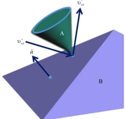
Figure 2 shows relation between two relative veloci- ties (rel
and rel
), before and after collision, is a resti- tution coefficient .
rel rel
(3)
The restitution coefficient must be satisfied to
0 1 If 1, then rel rel , and the collision is perfectly bouncy; in particular, no kinetic energy is lost. At the other end of the spectrum, 0 result in
0
rel
and a maximum of kinetic energy is lost [9]. General motion equations after collisions is
0
0
0
p t t t r
(4)
where r is fixed vector in body space, +, + and p are the linear velocity, rotational velocity and a general velocity of a particle after collision. By considering Equ- ations (1), (2) and (4) for each of bodies, and substituting them to the Equation (3), we derive impulse function in terms of the relative velocity before impact and restitu-tion coefficient [16].
1
1
0 0 0 0 0 0
1
1 1
ˆ ˆ ˆ ˆ
rel
a a a b b
a b
j
n t I t r n t r n t I t r n t r
M M
b
(5)
Here Ma and Mb are masses, Iaand Ib are inertia tensors
of the bodies, raand rb are relative radius of the contact
points of each body respect to mass of center [16].
The position extent of distance between virtual body surface and real body surface x is opposite proportiona- lity with the restitution coefficient value . The velocity of virtual body is a proportional relation to the restitu- tion coefficient . If assuming that body has no affection to distraction of kinetic energy, the virtual body surface and real body surface coincide (x = 0) therefore, there is no virtual velocity for the body ( = 0). If body is as- sumed with a great dissipation of kinetic energy then distance should be away from the surface of real body and virtual body velocity should be slow. Then it gives great value of T time.
Detailed derivation is in the reference [10]. Using this value and Equation (1), we simply determine the velocity after collision for each collision. In ODE, the restitution coefficient is given as constant for each collision. For the reality, this coefficient should be expressed close to the real world value.
5. The Graphical Method for Decision of
Restitution Coefficient
Figure 4 shows relation between restitution coefficient and time T which is spent by virtual bodies to reach at the contact point C2.
Physically, the restitution coefficient of bodies, which are in a collision, depends on their material property. In the real world, there is an energy loss, at least for generating sound, after impact of two bodies. This requires a proper assumption of modeling for the collision body in a com- puter graphic animation and robot simulation [17].
We show relation characteristics between restitution coefficient and virtual parameters in Figures 5 and 6 which are obtained by Equations (6) and (7).
Therefore we can choose virtual parameters by using characteristics that demonstrate the restitution coefficient for graphical animation of real bodies.
Our assumption for approximation of restitution coef- ficient consists of two parameters. First, we assume that each body (A1 and B1) has their own virtual body (A2 and
B2) and inside them (Figure 3). This virtual body’s sur- face has definite distance (xA and xB) from the real body’s
surface (Figure 3(a)). Next, virtual bodies A2 and B2 move to the contact point with the predetermined con- stant velocities A2 and B2 for individual body, when-
ever two real bodies get in a collision at the contact point
C1 (Figure 3(b)). The virtual body, with faster velocity and closer distance to the contacting point C1 reaches to the real body surface (in other words contacting point C1), at first (Figure 3(c)). Then it penetrates to the opposite body and consequently changes its velocity (VA2) to the
opposite virtual body’s velocity (VB2). It moves forward
until virtual bodies reach each other at the virtual body contact point C2. Thereafter, we calculate time T which is spent time by the motion of virtual bodies until they have a contact each other by using Equation (6).
6. Determining Virtual Body Characteristics
for Sport Game Balls
Official associations of sport games have their own stan- dards to test the ball quality that whether ball’s quality is adequate for using in a game or not. We collect these data from official sites of the games and the Table 1 shows the physical characteristics and testing characteri- stics for the balls. We choose the five kinds of sport ga- mes:
Basketball; Volleyball; Soccer (Football); Tennis;
Table tennis (Ping-Pong).
By assuming initial velocity in an initial height we can calculate velocities just before colliding and just after colliding. The initial velocity is zero when we drop ball test. Therefore, we can calculate final velocity as ball reaches floor.
2hg
(8) If we substitute (8) to (3), we find restitution coeffici- ent as follows.
h H
(9)
2 2 2 2 A B A B x x T
(6)
where xA and xB are the positions of the virtual bodies,
while A2 and B2 are velocities of the virtual bodies.
We can use this time value to determine the restitution coefficient (7).
KT
e
(7) where K is a real constant.
The combination of virtual body’s position and velo- city implies that there is a loss of kinetic energy in a col-lision.
Figure 3. An assumption of virtual body in the collision. (a) Two real bodies A1 and B1 move towards each other with
their own velocities
1
A and
1
B
.Virtual bodies A1 and B1
have their own initial distance xA and xB; b) Two bodies are
in a collision at the contact point C1; c) Since real bodies are
in a collision, virtual body A2 penetrates to surface of the real
body , but changes its velocity to the virtual body B2’s
velocity
1
B
2
B
[image:4.595.64.278.86.364.2] ; d) Two virtual bodies move towards each other with same velocity until they reach at the contact point C2 of virtual bodies.
Figure 4. The relation between restitution coefficientεand the collision time T of virtual bodies.
The floor has to be steel for the testing, this gives us opportunity to determine virtual characteristics for a ball. Under this condition, we can assume one body (steel floor) as it has no motion, and we can change (6) as follows:
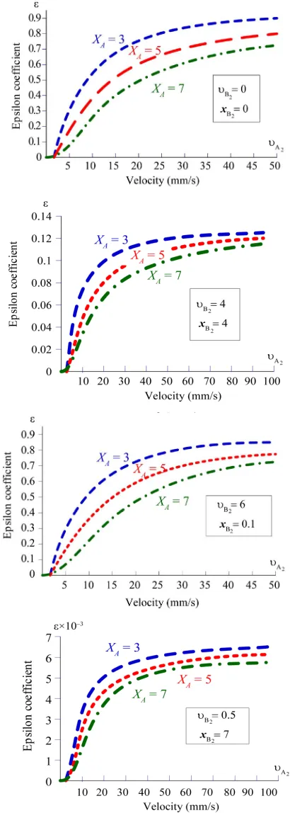
Figure 5. Here are the characteristics that demonstrate the relate to the velocity as for two colliding bodies. We give constant values to the position (xB) and velocity (B2) of the
virtual body B2. and three different values to the position
(xA) of the another virtual body A2 and vary the velocity
2
[image:4.595.69.282.501.647.2]
Figure 6. Here are the characteristics that demonstrate the restitution coefficient relate to the distance as for two colliding bodies. We give constant values to the position (xB) and velocity (B2) of the virtual body B2, and three different values to the
[image:5.595.77.535.287.544.2]velocity (A2) of the another virtual body A2 and vary the position xA.
Table 1. Physical and testing characteristics of sport game balls.
Bouncing height [m] Restitution coefficient
Sport games Mass [g] Circumference
[cm] Diameter [mm]
Dropping height
[m] min max min max
Basketball ball
(FIBA) 567 - 650 0.749 - 0.78 - 1.8 0.13 - 0.85 -
Volleyball ball 260 - 280 65 - 67 - 1.0 0.6 0.66 0.77 0.81
Soccer Football ball 420 - 445 68.5 - 69.5 - 2.0 0.12 1.65 0.77 0.9
Tennis ball 56 - 59.4 - 65.41 - 68.58 2.54 1.346 - 2.0 1.473 - 2.0 0.73 0.76
Table tennis ball 2.7 - 40 0.305 0.24 0.26 0.89 0.92
2 2
B
B x T
(10)
where xB is the virtual body’s position of the ball while 2
B
[image:5.595.351.496.580.710.2] is virtual velocity of the ball.
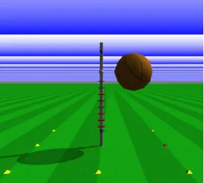
Figure 7 shows the relation between virtual velocity and virtual position of basketball ball. The basketball ball bouncing test in ODE environment is depicted in Figure 8. In the Table 2 we show parameters of selection for virtual velocity and virtual position by using Equations (7) and (10) for determine the restitution coefficient of some real balls in ODE.
Figure 7. The relation between virtual velocity and position of basketball ball.
7. Implementation in ODE
Previous section deals with an approximation for the re- stitution coefficient in the collision. In this section we discuss updating ODE with the restitution coefficient.
ODE creates a World for the dynamics calculation and Space for the collision detection. An object has two at- tributes which are a body for dynamics and a geometry for collision detection. A geometry attribute is defined by “Geom” structure on the simulation. Therefore we need to add information of virtual body to the structure “Geom” for the approximation. Two variables which are related to the position (x) and velocity () of the virtual body are added to the “Geom” structure. In ODE when collision occurs, ODE collision function approximates the
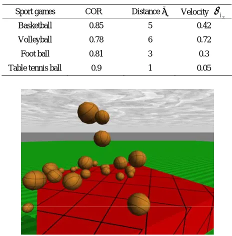
Table 2. Sample of selection for virtual velocity and virtual position of sport game balls.
Sport games COR ε Distance xA Velocity
2 A
Basketball 0.85 5 0.42
Volleyball 0.78 6 0.72
[image:6.595.55.287.111.347.2]Foot ball 0.81 3 0.3
Table tennis ball 0.9 1 0.05
Figure 9. Ball implementation in ODE with approximated restitution coefficient.
creates by using near Call back() function with o1 and o2 arguments for simulation [18]. In simulation the collision coefficient is calculated following algorithm.
For every contact ……….
Enable Contact Bounce Parameter Calculate Time constant T Calculate
……….
This algorithm helps us to decide restitution coeffici- ent for collision between many bodies related to their property of material. Figure 9 is the simulation results of bouncing bodies.
8. Conclusion
Open Dynamic Engine (ODE) is powerful and useful well-introduced physics engine for computer animation and robot simulation. Unfortunately, in ODE, restitution coefficient is assigned by the user for every collision. Even though, the restitution coefficient depends on many physical factors of each body which are in a collision, we have attempted to approximate this coefficient for ODE by using assumption of the virtual body, and its position and velocity. This assumption gives us better opportunity to approximate the restitution coefficient. We also, im- plemented this approximation to the ODE and received good result. In order to test the simple approximation for restitution coefficient we use sport game balls as models that has its standards by official associations. So, we can
see that the simple approximation is valid for collision, especially, for balls.
9. Acknowledgements
This work was supported by project of School of Infor- mation and Communications Technology, Mongolian Uni- versity of Science and Technology.
REFERENCES
[1] D. Evan and J. Hsu, “Extending Open Dynamics Engine for Robotics Simulation,” Springer-Verlag, Berlin, 2010. [2] http://opende.sourceforge.net
[3] S. Faik and H. Witteman, “Modeling of Impact Dyna- mics Literature Survey,” International ADAMS Users’
Conference, Orlando, 17-19 June 2000, pp. 3-10.
[4] T. Schwager and T. Pöschel, “Coefficient of Restitution and Linear-Dashpot Model Revisited,” Granular Matter, Vol. 9, No. 6, 2007, pp. 465-469.
doi:10.1007/s10035-007-0065-z
[5] M. Nagurka and S. G. Huang, “A Mass-Spring-Damper Model of a Bouncing Ball,” Proceedings of the 2004 Ame- rican Control Conference, Boston, 30 June-2 July 2004, pp. 499-504.
[6] X. Zhang and L. Vu-Quoc, “Modeling the Dependence of the Coefficient of Restitution on the Impact Velocity in Elasto-Plastic Collisions,” International Journal of Impact Engineering, Vol. 27, No. 3, 2002, pp. 317-341.
doi:10.1016/S0734-743X(01)00052-5
[7] D. W. Marhefka and D. E. Orin, “Simulation of Contact Using a Nonlinear Damping Model,” Proceedings of
IEEE International Conference on Robotics and Automa-tion, Minneapolis, 22-28 April 1996, pp. 1662-1668. [8] As Approved by FIBA Central Board, “Official Basket-
ball Rules 2010,” San Juan, 2010, pp. 2-81.
[9] C. J. Lu and M. C. Kuo, “Coefficients of Restitution Ba- sed on a Fractal Surface Model,” Journal of Applied Me-
chanics,Vol.70, No. 3, 2003, pp. 339-345. doi:10.1115/1.1574063
[10] J. Bender and A. Schmitt, “Constraint-Based Collision and Contact Handling Using Impulses,” Proceedings of
the 19thInternational Conference on Computer Anima-
tion and Social Agents, Geneva, 5-7 June 2006, pp. 3-11. [11] http://www.njp.org
[12] D. J. Wagg, “A Note on Coefficient of Restitution Mo- dels including the Effects of Impact Induced Vibration,”
Journal of Sound and Vibration, Vol. 300, No. 3-5, 2007, pp. 1071-1078.doi:10.1016/j.jsv.2006.08.030
[13] H. F. Frank, “Determination Coefficient of Restitution Based on Model Test Data,” Journal of Applied Mecha-
nics, Vol. 70, 2003, pp. 339-345.
[14] T. Lens, “Simulation of Dynamics and Realistic Contact Forces for Manipulators and Legged Robots with High Joint Elasticity,” 15th International Conference on
between Non Convex Objects Using a Nonlinear Damping Model,” International ADAMS User Conference, Ann Ar-bor, 9-10 June 1998, pp. 1-8.
[16] http://www.pixar.com/aboutpixar/research/pbm2001 [17] Ts. Khurelbaatar and B. Luubaatar, “The Graphical Me-