Local time variation in the large-scale structure of
1
Saturn’s magnetosphere
2
A. M. Sorba1,2, N. A. Achilleos1,2, N. Sergis3,4, P. Guio1,2, C. S. Arridge5, and 3
M. K. Dougherty6 4
1Department of Physics and Astronomy, University College London, London, UK. 5
2Centre for Planetary Sciences at UCL/Birkbeck, London, UK. 6
3Office for Space Research and Technology, Academy of Athens, Athens, Greece. 7
4Institute of Astronomy, Astrophysics, Space Applications and Remote Sensing, National Observatory of 8
Athens, Athens, Greece. 9
5Department of Physics, Lancaster University, Lancaster, UK. 10
6Space and Atmospheric Physics Group, Blackett Laboratory, Imperial College London, London, UK. 11
Key Points: 12
• We use hot plasma pressure observations to update the UCL/AGA model of
Sat-13
urn’s magnetodisk
14
• We investigate how local time variations in hot plasma and effective disk radius
15
influence the magnetic field structure
16
• We find variability in current sheet thickness, density and ionospheric field line
17
mappings
18
Abstract 19
The large-scale structure of Saturn’s magnetosphere is determined by internal and
ex-20
ternal factors, including the rapid planetary rotation rate, significant internal hot and
21
cold plasma sources, and varying solar wind pressure. Under certain conditions the
day-22
side magnetospheric magnetic field changes from a dipolar to more disk-like structure,
23
due to global force balance being approximately maintained during the reconfiguration.
24
However it is still not fully understood which factors dominantly influence this
behav-25
ior, and in particular how it varies with local time. We explore this in detail using a
2-26
D force-balance model of Saturn’s magnetodisk to describe the magnetosphere at
dif-27
ferent local time sectors. For model inputs, we use recent observational results which
sug-28
gest a significant local time asymmetry in the pressure of the hot (>3 keV) plasma
pop-29
ulation, and magnetopause location. We make calculations under different solar wind
30
conditions, in order to investigate how these local time asymmetries influence
magne-31
tospheric structure for different system sizes. We find significant day/night asymmetries
32
in the model magnetic field, consistent with recent empirical studies based onCassini
33
magnetometer observations. We also find dawn-dusk asymmetries in equatorial current
34
sheet thickness, with the varying hot plasma content and magnetodisk radius having
com-35
parable influence on overall structure, depending on external conditions. We also find
36
significant variations in magnetic mapping between the ionosphere and equatorial disk,
37
and ring current intensity, with substantial enhancements in the night and dusk sectors.
38
These results have consequences for interpreting many magnetospheric phenomena that
39
vary with local time, such as reconnection events and auroral observations.
40
1 Introduction
41
A magnetosphere is a magnetic and plasma structure that surrounds a magnetized
42
planet, due to the interaction between the planetary magnetic field and the solar wind.
43
At Saturn, the large-scale configuration of the magnetosphere is determined by a
num-44
ber of factors; the rapid (∼10.7 hour period) rotation rate of the planet (Desch & Kaiser,
45
1981), and significant internal plasma population originating from the cryovolcanic moon
46
Enceladus (Dougherty et al., 2006), give rise to a ‘disk-like’ magnetic field structure. In
47
the outer magnetosphere, beyond∼15 RS(where RS is Saturn’s radius, 60 268 km), the
48
magnetospheric magnetic field lines are radially stretched outwards in the equatorial plane
49
compared to a dipolar configuration. This is supported by an equatorial azimuthal ring
current, such that the associated magnetic pressure and curvature forces balance the
cen-51
trifugal force acting radially outwards on the rapidly rotating plasma. The centrifugal
52
force can be directly linked to an inertial current which contributes to the total ring
cur-53
rent; this inertial component is equivalent to the azimuthal drift associated with
centrifu-54
gal force in a frame corotating with the plasma. In the middle and outer magnetosphere,
55
beyond∼10 RS, there is also a significant population of hotter (>3 keV for ions) and 56
more variable plasma, which also contributes to the formation of a magnetodisk
struc-57
ture, via an enhancement of the ring current (Sergis et al., 2010). This relationship is
58
discussed in more detail in the next section via equation (1). In addition, pressure
bal-59
ance between the magnetosphere and the varying external solar wind pressure conditions
60
typically determines the approximate shape and size of the magnetosphere (Pilkington
61
et al., 2015a). Changes in magnetopause morphology in turn influences the internal
mag-62
netic field configuration. Both modeling and observational studies have shown that the
63
dayside magnetic field changes configuration to become more disk-like when the system
64
expands to a larger size (Achilleos, Guio, & Arridge, 2010; Arridge et al., 2008; Bunce,
65
Arridge, Cowley, & Dougherty, 2008; Sorba et al., 2017).
66
The relative importance of each of these factors in controlling Saturn’s
magneto-67
spheric structure is currently an area of active research. In recent years, a more global
68
understanding of Saturn’s magnetosphere has become possible largely thanks to the
ex-69
tensive temporal, spatial and seasonal coverage of theCassini space mission, which toured
70
the Saturnian magnetosphere from 2004 to 2017. In particular there is now an
oppor-71
tunity to investigate in more detail how the large-scale structure of Saturn’s
magneto-72
sphere varies withlocal time, and which factors control this behavior. This information
73
is important for interpreting a range of phenomena at Saturn; for example the likelihood
74
of reconnection events in different regions of the magnetosphere (Delamere, Otto, Ma,
75
Bagenal, & Wilson, 2015), which is related to how current sheet thickness varies with
76
local time (Kellett et al., 2011). Understanding more about the structure of the current
77
sheet is also important for studies of the observed periodicities at Saturn’s magnetosphere,
78
which investigate how the position and thickness of the equatorial current sheet are
mod-79
ulated at a period close to the planetary rotation rate (e.g. Cowley & Provan, 2017;
Thom-80
sen et al., 2017). More generally, a good picture of the global magnetic field structure
81
at different local times is important for understanding how different regions of the
netosphere magnetically map to the polar ionosphere in different local time sectors, for
83
example when interpreting observations of Saturn’s aurora.
84
A recent empirical study of magnetopause crossings by Pilkington et al. (2015b)
85
showed evidence of a dawn-dusk asymmetry in the location of the magnetopause
bound-86
ary, while a survey of magnetospheric plasma populations from Sergis et al. (2017) showed
87
significant local time asymmetry in the hot plasma population, with enhanced pressures
88
in the dusk and midnight local time sectors compared to dawn and noon. These factors
89
will influence the magnetic and plasma configuration of the magnetosphere differently
90
at different local times. In addition, a recent magnetic field model by Carbary (2018)
91
shows significant day-night asymmetry in equatorial-ionospheric magnetic mapping
pro-92
files, and local time asymmetries in the location of Saturn’s aurora have been observed
93
in studies such as Badman et al. (2011); Badman, Cowley, G´erard, and Grodent (2006).
94
In this work we investigate the relative importance of these factors in controlling
95
magnetospheric structure at different local time sectors using a modeling approach, to
96
complement observational studies. We use the University College
London/Achilleos-Guio-97
Arridge (UCL/AGA) model, a 2-D force-balance magnetic and plasma model of Saturn’s
98
magnetodisk from Achilleos, Guio, and Arridge (2010). We adapt this model to describe
99
the typical, equilibrium conditions of Saturn’s magnetosphere at four different local time
100
sectors; noon (09:00-15:00), dawn (03:00-09:00), dusk (15:00-21:00) and night (21:00-03:00).
101
We use equatorial profiles of the hot plasma pressure from Sergis et al. (2017) for the
102
different local time sectors as boundary condition inputs to the magnetodisk model, and
103
determine appropriate magnetopause radius values to use for each sector based on the
104
magnetopause surface model of Pilkington et al. (2015b). Our method of constructing
105
these models is described in Section 2. In Section 3 we present the results of these
cal-106
culations, and highlight interesting comparisons in the magnetic field structure, azimuthal
107
current density and magnetic mappings for the different local time sectors. Section 4
pro-108
vides a brief summary of the main conclusions of this work.
109
2 Method
110
2.1 The UCL/AGA Force-Balance Magnetodisk Model 111
In this study we used a modified version of the UCL/AGA magnetic field and plasma
112
model first described by Achilleos, Guio, and Arridge (2010), itself based on a model
inally constructed for the Jovian magnetodisk by Caudal (1986), adapted for Saturn. More
114
information can be found in those studies. The model is axisymmetric about the
plan-115
etary dipole/rotation axis, which are assumed to be parallel. This parallel assumption
116
is appropriate for Saturn in particular, as the rotation and dipole axes are aligned to within
117
0.01◦ (Dougherty et al., 2018). This axisymmetric assumption is appropriate as an
ap-118
proximation of the large-scale structure of the magnetic field, as shown by Hunt et al.
119
(2014), who compared the gradients of currents in radial, azimuthal and meridional
di-120
rections and found the azimuthal gradients could be neglected. The model is constructed
121
based on the assumption of force balance in the rotating plasma of the magnetosphere
122
between the Lorentz body force (magnetic pressure and tension forces), pressure
gradi-123
ent force and centrifugal force, such that
124
J×B=∇P−nmiω2ρˆρ (1)
125
whereJ is the current density,B is the magnetic field vector andρis cylindrical radial
126
distance from the rotation/dipole axis, withρˆits unit vector. The plasma properties are
127
isotropic pressureP, ion number densityn, mean ion massmi and angular velocityω.
128
Equatorial radial profiles of these plasma properties are required boundary conditions
129
for this model and were obtained from studies based on observations from theCassini
130
plasma instruments CAPS (CAssini Plasma Spectrometer, Young et al., 2004) and MIMI
131
(Magnetospheric IMaging Instrument, Krimigis et al., 2004). These are presented in Achilleos,
132
Guio, and Arridge (2010) and updated for this study as described in the following
sec-133
tions. The equatorial radial profile of angular velocityω necessary to calculate the
cen-134
trifugal force term was obtained using a recent study of CAPS observations from
Wil-135
son, Bagenal, and Persoon (2017), as described in Sorba et al. (2018). The plasma is
as-136
sumed to consist of a cold population with pressurePC, confined towards the
equato-137
rial plane due to the centrifugal force exerted on it, and a hot population with
associ-138
ated pressurePH distributed uniformly along magnetic field lines. 139
Any magnetic field can be represented in terms of two Euler potentialsαandβ,
140
B=∇α×∇β, as a consequence of magnetic fields being divergence-free (Stern, 1970).
141
For an axisymmetric field with no azimuthal component, the forms ofαandβ can be
142
chosen such that all information about the poloidal field is contained in one Euler
po-143
tential, which we callα, which is constant along magnetic field lines. Caudal (1986) showed
144
that equation (1) corresponds to a partial differential equation which can be solved
it-145
eratively forα, providing magnetic field and plasma distributions as a function of
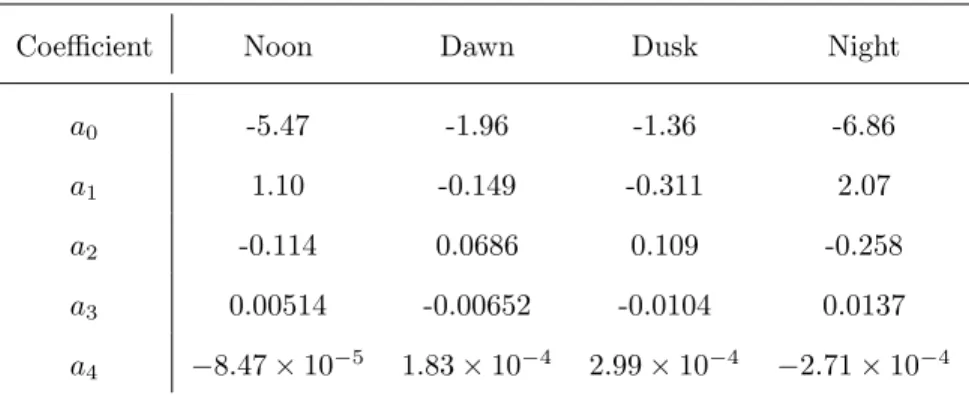
Table 1. Coefficients of fourth order polynomial fits to the logarithm of each of the hot pres-sure profiles shown in Figure 1, as described in the main text.
156
157
Coefficient Noon Dawn Dusk Night
a0 -5.47 -1.96 -1.36 -6.86
a1 1.10 -0.149 -0.311 2.07
a2 -0.114 0.0686 0.109 -0.258
a3 0.00514 -0.00652 -0.0104 0.0137
a4 −8.47×10⁻⁵ 1.83×10⁻⁴ 2.99×10⁻⁴ −2.71×10⁻⁴
drical radial distanceρ, and height with respect to the rotational equatorz. We say that
147
the model has achieved convergence when the relative difference inαbetween two
suc-148
cessive iterations falls below 0.5%, when using the mean of the current and previous
so-149
lutions at each iteration (see detailed discussion about this numerical relaxation in Sorba
150
et al., 2018).
151
This model was originally used to represent typical dayside conditions at Saturn,
152
and so we made various modifications described herein, which are necessary to
appro-153
priately represent different local time sectors.
154
2.2 Hot Plasma Parameterization for Different Local Time Sectors 155
An important boundary condition for this model is the equatorial profile of hot plasma
162
pressure. It was shown by Achilleos, Guio, Arridge, Sergis, et al. (2010) that variations
163
in this quantity estimated using the spread of observations from e.g. Sergis et al. (2007)can
164
have a significant impact on the magnetic field configuration of a typical dayside model.
165
In Achilleos, Guio, Arridge, Sergis, et al. (2010), the authors used quartile fits to
equa-166
torial hot (> 3keV) plasma pressure observations fromCassini MIMI to show that a
167
globally elevated hot plasma pressure and associated pressure gradient causes a more
disk-168
like magnetic field structure, with more radially stretched field lines, due to the
enhance-169
ment of the equatorial ring current. Achilleos, Guio, Arridge, Sergis, et al. (2010) also
170
found that variations in the hot plasma content affected magnetic mapping between the
171
equatorial disk and the ionosphere. As discussed in Section 1, the magnetospheric hot
6 8 10 12 14 16
Radial Distance (RS)
10-2 10-1
Hot Pressure (nPa)
Noon Dawn Dusk Night
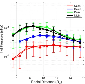
Figure 1. Equatorial radial profiles of hot plasma pressure for different local time sectors, as shown by the color. Solid circles and error bars are means and standard errors for binned data from Sergis et al. (2017), and solid lines are 4th order polynomial fits to the logarithms of the data points, as described in the main text.
158
159
160
161
plasma population also affects the compressibility of the magnetopause and overall
force-173
balance (Sorba et al., 2017).
174
More recently, a comprehensive study usingCassini MIMI data (Sergis et al., 2017)
175
showed that the pressure of this hot plasma population not only varies over time and
176
distance, but also varies significantly with local time, even when averaged over a large
177
portion of theCassini mission (July 2004 - December 2013). Sergis et al. (2017) also found
178
that especially in the middle and outer magnetosphere beyond∼11 RSpressure
gradi-179
ents associated with both hot and cold populations contributed more to the total ring
180
current than centrifugal acceleration, except in the noon sector where both contributed
181
approximately equally. Therefore in this study, we used average equatorial profiles of hot
182
plasma pressure between 5 and 16 RSpresented in Sergis et al. (2017) for the different 183
local time sectors, as boundary conditions for our models. Specifically, we fit the 1 RS -184
width-binned data presented in Sergis et al. (2017) using polynomial functions of the form
185
log(PH) =a0+a1ρ+a2ρ2+a3ρ3+a4ρ4 (2)
following the approach used in Sergis et al. (2017), with each point weighted by the
in-187
verse square of the provided standard error of the mean. The resulting coefficients for
188
each sector are shown in Table 1, with pressure in units of nPa and radial distance in
189
units of RS. The polynomials are shown in Figure 1, as well as the corresponding ob-190
servations from Sergis et al. (2017), with standard error of the mean of each bin shown
191
by the error bars. This figure shows that the hot plasma pressure is significantly higher
192
in the dusk and night sectors than the dawn and noon sectors. Here the dawn, noon, dusk
193
and night sectors are defined by the magnetic local time intervals 03:00-09:00, 09:00-15:00,
194
15:00-21:00 and 21:00-03:00 respectively.
195
For values ofρsmaller than the applicable range of the polynomials (5.5 RS) we 196
assumed the hot plasma pressure falls linearly to zero withρ, broadly in line with
ob-197
servations and with the approach of Achilleos, Guio, and Arridge (2010). For the dawn
198
profile we used an inner boundary of 6.5 RSdue to lack of data in the innermost bin in 199
the Sergis et al. (2017) data, which can be seen in Figure 1. For values ofρabove the
200
applicable range of the polynomials (15.5 RS), we assumed a profile where the product 201
of the hot plasma pressure and the local flux tube volume is constant with radial
dis-202
tance, following previous studies such as Achilleos, Guio, and Arridge (2010); Sorba et
203
al. (2017). In practice for the dawn and dusk models we used outer limits of 15.3 RSand 204
15.1 RSrespectively, which are the locations of the local minima in the hot pressure poly-205
nomials, to ensure a smoother profile.
206
2.3 Magnetopause Radius for Different Local Time Sectors 207
The UCL/AGA magnetodisk model used in this work can also be parameterized
212
by an effective disk radiusRD, the equatorial radial distance of the last closed field line
213
in the model. As discussed in Section 1, variations in this quantity also significantly
im-214
pact the resulting magnetic field structure in the model, with more expanded systems
215
(largerRD) having a more disk-like magnetic field structure, i.e. more radially ‘stretched’ 216
field lines (e.g. Achilleos, Guio, & Arridge, 2010; Sorba et al., 2017). This relationship
217
is due to overall force balance in the magnetosphere requiring a larger magnetic tension
218
force with a smaller radius of curvature for more expanded systems. This is also seen in
219
observational studies such as Arridge et al. (2008), who find that in the noon sector,
Sat-220
urn’s magnetosphere only shows a significant divergence from a dipolar field structure
221
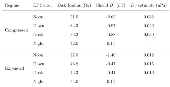
Table 2. Configuration details for the two families of models used to represent different local time sectors, for compressed (high solar wind dynamic pressure) and expanded (low solar wind dynamic pressure) regimes. Magnetodisk radius, shielding magnetic field value and an estimate for the solar wind dynamic pressureDPare shown for each model.
208
209
210
211
Regime LT Sector Disk Radius (RS) ShieldBz(nT) DP estimate (nPa)
Compressed
Noon 21.0 -2.62 0.032
Dawn 34.3 -0.97 0.026
Dusk 33.2 -0.88 0.030
Night 42.0 0.14
-Expanded
Noon 27.0 -1.40 0.012
Dawn 43.8 -0.47 0.015
Dusk 42.3 -0.41 0.016
Night 54.0 0.13
-netodisc structure is consistently observed on the flanks and nightside, where the
mag-223
netopause radius is greater.
224
It was therefore important for this work that we chose appropriate values of the
225
disk radiusRD for each of the local time sectors we were describing. To do this, we
ap-226
pealed to the study of Pilkington et al. (2015b), who improved the earlier Saturn
mag-227
netopause surface models of Arridge, Achilleos, Dougherty, Khurana, and Russell (2006);
228
Kanani et al. (2010); Pilkington et al. (2015a) by in particular including a small
dawn-229
dusk asymmetry in magnetopause radius in the model. In Pilkington et al. (2015b) the
230
authors used observations of magnetopause crossings made throughout a large portion
231
of theCassini mission to constrain parameters for a Shue et al. (1997) type magnetopause
232
model, introducing an extra parameter to describe the dawn-dusk asymmetry. They found
233
that on average the magnetopause boundary extends farther from the planet on the dawn
234
side than the dusk side, by∼7%. The authors suggested this may be due to a
combi-235
nation of factors including asymmetries in internal pressure populations, and intrinsic
236
asymmetry in plasma flow around the planet with respect to the direction of solar wind
237
flow, with the flows in approximately opposite directions at dawn pushing the
magne-238
topause further out in this sector.
In order to investigate how local time variation in magnetospheric structure varies
240
with system size, we calculated two sets of models under different solar wind dynamic
241
pressure conditions; a compressed regime with subsolar magnetopause radius fixed at 21 RS, 242
and an expanded regime with subsolar magnetopause radius fixed at 27 RS, following the
243
bimodal values observed in Pilkington et al. (2015a) and Achilleos et al. (2008). For the
244
corresponding dawn and dusk disk radii, we calculated the magnetopause radius at the
245
center of each local time sector (06:00 for dawn and 18:00 for dusk) using the best fit
pa-246
rameters given in Pilkington et al. (2015a) and Pilkington et al. (2015b). We used a value
247
of the nose plasmaβ = 3 (whereβ is the ratio of plasma pressure to magnetic
pres-248
sure), which is the median value for the dataset quoted in Pilkington et al. (2015a),
al-249
though for a fixed subsolar radius this choice ofβ had very little impact on the
result-250
ing flank radii. Thus we determined the appropriate disk radiiRD for noon, dawn and
251
dusk local time sectors, for both high and low solar wind pressure conditions. The
re-252
sulting values are shown in Table 2. In the absence of an accurate magnetopause model
253
for the nightside of Saturn’s magnetosphere, we used a disk radius of twice the
subso-254
lar magnetopause radius to represent an approximate nightside local time sector
struc-255
ture.
256
The solar wind dynamic pressure corresponding to a given equilibrium magnetodisk
257
model can be estimated by assuming pressure balance across the boundary at the
equa-258
tor, as in Sorba et al. (2017). Specifically we can assume
259
B2 MS
2µ0
+PMS=
kcos2(ψ) + kBTSW 1.16mpu2SW
sin2(ψ)
DP (3)
260
where terms on the left hand side represent the magnetospheric (hence MS subscript)
261
magnetic and plasma pressures just inside the magnetopause boundary, and the terms
262
on the right (the coefficients of upstream solar wind dynamic pressureDP) represent the
263
component of solar wind dynamic pressure incident on the magnetopause surface, and
264
a smaller component associated with the solar wind’s thermal pressure. k = 0.881 is
265
a factor to account for the diversion of flow around the magnetosphere obstacle (see
Spre-266
iter, Alksne, & Abraham-Shrauner, 1966),TSW anduSW are the temperature and speed
267
of the solar wind, andψis the angle between the incident solar wind and the magnetopause
268
surface normal. This same relationship was also used in Pilkington et al. (2015a) to
es-269
timate solar wind dynamic pressure based on internal magnetospheric observations, and
270
was initially proposed in this form by Kanani et al. (2010), based on the original
formu-271
lation by Petrinec and Russell (1997).
We used values forBMS andPMS = PH+PCextracted just inside the magne-273
topause boundary of each model, and obtainedψfrom the Pilkington et al. (2015a)
mag-274
netopause surface model at the appropriate local time sector. Finally, we assumed
typ-275
ical parameterskBTSW = 100 eV anduSW = 460 km s−1 following Pilkington et al.
276
(2015a). The resulting estimates ofDP are shown in Table 2. This approach is not
ap-277
propriate for the far night-side tail, where a concept ofψis not directly applicable, and
278
so we do not attempt to estimateDP for those sector models. While the values ofDP
279
do not exactly agree for all compressed or all expanded models, we can see that the two
280
regimes provide significantly different, self-consistent estimates; the meanDP estimates
281
are 0.029±0.003 nPa and 0.014±0.002 nPa for the compressed and expanded regimes
282
respectively. Therefore our two families of models, compressed and expanded, broadly
283
correspond to systems under different solar wind conditions, whilst representing
typi-284
cal internal conditions.
285
It is also interesting to note that there is evidence that Saturn’s magnetopause
bound-286
ary position is periodically modulated at a rate close to planetary rotation rate,
inde-287
pendent of changes in incident solar wind dynamic pressure. This was first suggested by
288
Espinosa and Dougherty (2001) and Espinosa, Southwood, and Dougherty (2003) based
289
on observations fromPioneer 11 magnetic field data. Later, Clarke, Andrews, Arridge,
290
Coates, and Cowley (2010) analysedCassini magnetometer (MAG) (Dougherty et al.,
291
2004) and CAPS electron spectrometer data and found that Saturn’s dayside magnetopause
292
was periodically displaced by up to 5 RSin the post-noon local time sector, associated 293
with rotating perturbations in internal magnetic field and plasma properties.
Magne-294
tohydrodynamic (MHD) simulations of Saturn’s magnetosphere presented in Kivelson
295
and Jia (2014) showed similar behavior, with constant solar wind properties in their
mod-296
els such that the observed perturbations were again driven by periodic perturbations in
297
internal processes. Kivelson and Jia (2014) and later Ramer, Kivelson, Sergis, Khurana,
298
and Jia (2017) explored how this modulation in magnetopause position may vary across
299
local time sectors, and found a complicated relationship between the phase of the
rotat-300
ing perturbation and its effect on the magnetosphere morphology depending on the
lo-301
cal time.
302
Varying the magnetopause radius in such a way would affect the magnetic field and
303
plasma properties predicted by our magnetodisk models for a given local time sector,
sim-304
ilarly to how our model predictions vary for compressed and expanded regimes (as
cussed later in this study). In Sorba et al. (2018), the authors used forms of the UCL/AGA
306
magnetodisk model to try and characterize these periodic perturbations inCassini
mag-307
netic field data in the outer magnetosphere around the dusk sector. They used a
fam-308
ily of magnetodisk models calculated at different magnetopause radii and organised with
309
planetary longitude (but not local time) to represent a rotational perturbation in
cur-310
rent sheet thickness, with a thicker current sheet represented by a model with a smaller
311
magnetodisk radius. As in this study, Sorba et al. (2018) calculated that the estimated
312
effective solar wind dynamic pressure associated with each magnetodisk model was
dif-313
ferent and so the family of models did not represent a system under constant solar wind
314
dynamic pressure. However Sorba et al. (2018) found that their approach could still
char-315
acterize the phase and amplitude of the perturbations particularly in the meridional
com-316
ponent of the magnetic field data. A deepened understanding of how the large-scale
struc-317
ture of Saturn’s magnetosphere varies across local time would further help with future
318
studies of this nature.
319
2.4 Magnetodisk Model Adaptations 320
Finally, we made minor adaptations to the magnetodisk model construction in
or-321
der to be more appropriate for different local time sectors. In Achilleos, Guio, and
Ar-322
ridge (2010) the authors include a small, uniform, southward-directed ‘shielding field’
323
to the total magnetic field at every iteration, to approximately account for the magnetic
324
field associated with the magnetopause and magnetotail current sheets. The magnitude
325
of this field was chosen by calculating dayside equatorial averages of the empirical field
326
models of Alexeev and Belenkaya (2005) and Alexeev et al. (2006), and it varied with
327
model magnetodisk radiusRD (see Achilleos, Guio, & Arridge, 2010, Figure 6). For this
328
study, we calculated local time sector averages of these field models over circular segments
329
with radiusRD, to account for the increased significance of the tail current field
com-330
pared to the magnetopause current field for nightside local time sectors in particular. We
331
also enhanced the field associated with the magnetopause current beyond a dipole
ap-332
proximation by a factor (1+kMD), wherekMDis the ratio of the ring current and plan-333
etary dipole magnetic moments, as in Sorba et al. (2018), following Alexeev and Belenkaya
334
(2005). As in Sorba et al. (2018), to estimate the appropriatekMD for each model we
335
employed an extrapolation of the empirical linear fit from Bunce et al. (2007), although
336
here we used our values ofRD rather than the subsolar magnetopause radius to estimate
kMDas we found that this in particular improved convergence in our models. The re-338
sulting values for the shielding magnetic fieldBz for each model are shown in Table 2.
339
It can be seen that, as expected, the total shielding field decreases and becomes
north-340
ward directed for the nightside models due to the increased influence of the more
north-341
ward field associated with the distant tail currents, compared to the more southward field
342
associated with magnetopause currents. While the use of these shielding field values does
343
not significantly affect the global magnetic field structure of the resulting models, we find
344
it does improve the ability for our models to achieve convergence as defined above,
com-345
pared to model calculations using the same system size and hot plasma content
param-346
eters but the approach of Sorba et al. (2018).
347
We also updated the representation of the cold equatorial ion temperatures used
348
as a boundary condition in the magnetodisk model, using a recent comprehensive
sur-349
vey of equatorialCassini CAPS observations from Wilson et al. (2017). We fit the
equa-350
torial profiles of parallel and perpendicular temperatures for hydrogen and water group
351
ions between 5.5 and 30 RSpresented in Wilson et al. (2017) with fourth order polyno-352
mials, with points weighted by the inverse square of the error (assumed to be half the
353
interquartile range of each bin). We then derived a single equatorial plasma
tempera-354
ture profile for the magnetodisk model as in Achilleos, Guio, Arridge, Sergis, et al. (2010),
355
who used the same approach but with earlier more restricted data sets from Wilson et
356
al. (2008) and McAndrews et al. (2009). The best fit polynomials for each ion species
357
and temperature moment are given in the Supporting Information. We found that this
358
update using a much more comprehensive data set did not significantly affect the
over-359
all resulting magnetic field profile of the magnetodisk model, in general causing only a
360
slight increase in magnetic field strength in the inner magnetosphere, and slight decrease
361
in the outer magnetosphere, with a maximum difference under 1 nT. However this
up-362
date did improve model estimates of the cold plasma pressure, reducing the values in the
363
outer magnetosphere such that they showed better agreement with recent observations
364
from Sergis et al. (2017) (also based on CAPS data). This modification is an
improve-365
ment resulting from better radial coverage and global constraint of the cold plasma
tem-366
perature than in previous studies.
0 10 20 30 40 50 60
Radial Distance (R
S) 100 101 102 103 104 105
Equatorial B (nT)
Compressed Regime Noon Dawn Dusk Night (Dipole)
0 10 20 30 40 50 60
Radial Distance (R
S) 100 101 102 103 104 105
Equatorial B (nT)
Expanded Regime Noon Dawn Dusk Night (Dipole)
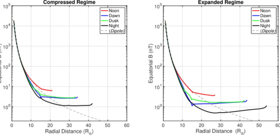
Figure 2. Equatorial profiles of total magnetic field strengthB with radial distance for each local time sector as shown by the color, for both the compressed (a) and expanded (b) regimes. On each plot a profile for a dipole magnetic field is shown in dashed grey for comparison.
374
375
376
3 Results and Discussion
368
3.1 Magnetic Field Structure 369
The equatorial magnetic field profiles from the resulting magnetodisk models for
370
each local time sector are shown in Figure 2. For comparison, a representative profile
371
for the internal planetary dipole magnetic field is shown by the grey dashed line on each
372
plot.
373
For the dayside (noon) models, we can see that the magnetic field is approximately
377
dipolar in the inner (.10 RS) magnetosphere, and falls more slowly with radial distance 378
than a dipole in the middle (10.ρ.15 RS) and outer magnetosphere. This
behav-379
ior broadly corresponds to a more ‘disk-like’ magnetic field structure compared to a dipole,
380
and appears for a more significant range in radial distance for the expanded noon model.
381
Similar behavior has been found in observational studies of Saturn’s magnetosphere. For
382
example Arridge et al. (2008) showed that the dayside magnetospheric magnetic field
383
was approximately dipolar when the system was compressed, but more disk-like when
384
expanded, particularly beyond a sub-solar magnetopause radius of∼23 RS. Results of 385
ring current modeling from Bunce, Arridge, Cowley, and Dougherty (2008) found a
sim-386
ilar result. This behavior is expected is a consequence of conservation of magnetic flux
387
threading the equatorial plane of the magnetosphere, such that compressing the system
necessarily increases the total magnetic field strength inside the magnetosphere as field
389
lines are pushed together, corresponding to a more dipolar configuration.
390
For the larger dawn, dusk, and night sector models, the model magnetic field strengths
391
are lower than the corresponding dipole field in the inner magnetosphere, and greater
392
in the outer magnetosphere. This too is in line within situ observations of Saturn’s
mag-393
netosphere, such as Delamere et al. (2015), who analyzed equatorial current sheet
cross-394
ings usingCassini MAG data in order to demonstrate how the equatorial magnetic field
395
varies with radial distance in different local time sectors. There is also a small dawn-dusk
396
asymmetry in the magnetic field strengths in our model, with the dusk sector profile
per-397
sistently higher than the dawn. This is likely due to the asymmetry in magnetopause
398
radius across the sectors, with a larger magnetic field strength at dusk associated with
399
the more compressed system there. This may also be partially associated with the higher
400
hot plasma pressure and associated gradient in the dusk sector requiring a greater
mag-401
netic curvature force to balance it. This is interesting to note, as such a small
asymme-402
try in field strength would be unlikely to reveal itself in observational studies of Saturn’s
403
magnetosphere, especially due to the relatively poor sampling of the dawn sector
equa-404
torial magnetosphere by theCassini spacecraft over its mission. Previous studies using
405
the UCL/AGA model have not investigated local time variations specifically; however
406
it was shown in Achilleos, Guio, and Arridge (2010), Achilleos et al. (2014) and Sorba
407
et al. (2018) that this type of model can characterize well the magnetic field measured
408
byCassini along some individual trajectories, especially when the periodic perturbations
409
in the current sheet are accounted for.
410
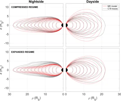
Looking at the day-night asymmetry in more detail, in Figure 3 we show the
mag-411
netic field structure for our noon and nightside magnetodisk models, for the compressed
412
(top panel) and expanded (bottom panel) regimes in the rangeρ= 4−22 RSfor the
day-413
side andρ= 4−28 RSon the nightside, noting that our compressed dayside model only
414
extends out toρ = 21 RS. For comparison, we include in gray field line traces based 415
on empirical observations from a recent study by Carbary (2018). In that study the
au-416
thor binned magnetic field observations from almost the entireCassini mission
[2004-417
2016] into two local time sectors, dayside and nightside, and calculated traces using a
418
Runge-Kutta propagator (see Carbary, 2018, and references therein for more details).
419
Carbary (2018) accounted for seasonal warping of the current sheet via a coordinate
trans-420
formation, however their model did not account for a change in external solar wind
ditions, and so we have reproduced the same traces from Carbary (2018) in the top and
422
bottom panels. We can see that the overall magnetic field structures in our models are
423
similar to those of the Carbary (2018) model, in particular the expanded 27 RSdayside
424
model, and the compressed 42 RSnightside model. Our expanded nightside model shows
425
a magnetic field structure that is significantly more disk-like than the Carbary (2018)
426
analytical model, suggesting that perhaps a magnetodisk radius of 54 RSis somewhat
427
too extreme to accurately characterize the typical midnight magnetosphere. In addition
428
our compressed dayside model has a significantly more dipolar structure than the
Car-429
bary (2018) model results. We should note that here we are comparing specifically our
430
noon (LT 09:00-15:00) and night (LT 21:00-03:00) sector models with the Carbary (2018)
431
traces which correspond to wider, 12 hour local time regions. Therefore to more
accu-432
rately represent (for example) the entire dayside for a more direct comparison, we would
433
need to consider some combination of our noon, dawn and dusk sector model outputs.
434
This makes it difficult to assess which approach gives a better overall representation of
435
the true Saturn magnetosphere system. However it can be seen that both our models
436
and the Carbary (2018) results show a transition from a more dipolar magnetic field
con-437
figuration when compressed on the dayside to a more stretched, disk-like configuration
438
on the nightside.
439
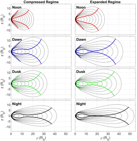
In order to investigate more just how ‘disk-like’ the magnetic field is in each local
446
time sector, we use a visualisation technique employed in Bunce, Arridge, Cowley, and
447
Dougherty (2008), itself based on the analytical approach in Arridge et al. (2008). For
448
each model we bound regions of the magnetosphere where the local magnetic field
di-449
rection lies within 30◦ of theρˆvector direction such that the field lines are approximately
450
parallel to the equatorial plane. The results are shown in Figure 4, and the
reproduc-451
tion of the most lower latitude of the bounding lines are shown in Figure 5. The
mag-452
netic field structure for each model is also shown in black, to further illustrate how this
453
method characterizes the ‘disky-ness’ of the magnetic field structures. These figures show
454
that, as expected, the larger magnetodisk models have significantly more disk-like
mag-455
netic field structures in the middle magnetosphere, than the smaller, more dipolar
mod-456
els. As discussed in the introduction, this was observed in previous studies such as Achilleos,
457
Guio, and Arridge (2010); Arridge et al. (2008); Sorba et al. (2017) and is a result of how
458
the overall force-balance within the magnetosphere changes with system size, in terms
459
of the dominant magnetic and plasma related forces.
Figure 3. A comparison of model magnetic field lines from Carbary (2018) and this study. In grey are shown traces based on binnedCassini magnetometer meridional magnetic field obser-vations from Carbary (2018) (top and bottom panels an exact reproduction). In red are shown magnetic field lines from the noon and nightside models presented in this study, for the com-pressed (top panel) and expanded (bottom panel) regimes, for L shells to match those of the Carbary (2018) study.
440
441
442
443
444
Figure 4. The magnetic field structure for each magnetodisk model for the compressed (left column) and expanded (right column) regimes, shown by the solid black lines. Superposed in color for each model are pairs of lines in each hemisphere which bound regions where the local magnetic field direction lies within 30◦of theρˆvector direction.
461
462
463
464
Figure 5. Reproduction of the more equatorward colored lines from Figure 4, for each local time sector model, for compressed (left) and expanded (right) regimes. These represent the low latitude boundaries of regions where the local magnetic field direction lies within 30◦of theρˆ
vector direction.
465
466
467
In addition, from Figure 5 in particular, it can be seen that, for the compressed regime,
469
the dusk sector has a slightly thinner and more disk-like magnetodisk structure in the
470
middle magnetosphere than the dawn sector, as shown by the bounding lines being more
471
equatorward for the dusk model (shown in green). This effect is likely due to the local
472
enhancement of the ring current in the dusk sector due to the increased hot plasma
pres-473
sure, which causes a more extreme perturbation from a dipolar magnetic field. This was
474
also discussed in the introduction, and observed in Achilleos, Guio, Arridge, Sergis, et
475
al. (2010); Sorba et al. (2017). Note that this ‘thinning’ of the disk is not the same as
476
thinning of theplasma sheet, which is made up of both hot and cold plasma populations.
477
While thecurrent sheet and associatedcold plasma sheet thins, the hot plasma is
ac-478
tually more populous for the thinner, dusk model, and the associated hot plasma
pres-479
sure is constant along magnetic field lines. The pressure distribution is also affected by
480
particle temperature, or more generally velocity distribution of particles. As described
481
in Arridge et al. (2009); Sergis et al. (2011) the current sheet, a predominantly magnetic
482
structure, has been observed to be thinner than the plasma sheet it is embedded in, and
483
the plasma sheet itself can have different thicknesses in different particle energies and
484
species.
485
For the expanded regime, it can be seen in Figure 5 that the opposite relationship
486
is true; in the middle and outer magnetosphere, the dawn sector magnetic field has a
thin-487
ner and more disk-like structure (shown in blue) than the dusk sector magnetic field (shown
488
in green). This is likely associated with the increased influence of the dawn-dusk
asym-489
metry in effective magnetodisk radius for the expanded regime, as a larger magnetopause
490
radius also promotes a more disk-like structure. For the expanded regime, the dawn
mag-491
netopause is 1.5 RS greater than the dusk, compared to 1.1 RS for the compressed regime. 492
It is interesting that this transition in dominant behavior occurs across this
compressed-493
expanded regime threshold. These results suggest that the asymmetries in magnetopause
494
radius and hot plasma content have comparable influence on the global magnetic field
495
structure in those local time sectors. In addition, the expanded system models may be
496
more strongly influenced by the assumption we made that the product of flux tube
vol-497
ume and hot plasma pressure is constant beyond 15.5 RS, as described in Section 2.2, 498
as this region is by definition more extended for the expanded system models, whereRD
499
is greater. We hope to relax this assumption with an updated parameterization of the
500
In order to more fully understand the significance of these observed differences
be-502
tween the dawn and dusk configurations, it would be helpful to estimate uncertainties
503
on the positions of these bounding lines. This could involve calculating an ensemble of
504
models with slightly varying input boundary conditions, or perhaps calculating models
505
to varying numbers of iterations, and comparing the outputs. While beyond the scope
506
of this study, this could be pursued in future.
507
In the aforementioned study by Delamere et al. (2015), the authors find significantly
508
more incidences of ‘critically thin’ equatorial current sheet encounters in the dusk
sec-509
tor than the dawn sector, even when accounting for the sampling bias ofCassini (which
510
spent more time in the dusk sector). This is therefore perhaps more in line with our
pic-511
ture of the compressed regime, with a thinner current sheet on the dusk side due to the
512
influence of the increased hot plasma pressure. However in general Delamere et al. (2015)
513
observe that the current sheet is only uniformly thin in the 0:00-6:00 ‘pre-dawn’ local
514
time sector, and that in all other sectors the observed meridional magnetic field strength
515
at the current sheet center shows significant variability, with perhaps stronger average
516
magnetic field strengths observed in the post-noon local time sector. In a study from Jia
517
and Kivelson (2016), based on MHD simulations of Saturn’s magnetosphere from Jia,
518
Hansen, et al. (2012), they find a significantly thinner current sheet and more radially
519
stretched magnetic field lines in the dawn sector, which is also observed at Jupiter (e.g.
520
Khurana et al., 2004). This may be understood, as that the simulations of Jia, Hansen,
521
et al. (2012) do not include a suprathermal plasma population, and so the effect of the
522
enhanced hot plasma population on the dusk side is not captured in their study. In
ad-523
dition, it was suggested by Pilkington et al. (2015b) that this absence of suprathermal
524
plasma in the Jia, Hansen, et al. (2012) models may cause their models to slightly
over-525
estimate the dawn-dusk asymmetry in magnetopause radius, which predict a mean
asym-526
metry of 2.6 RS, compared to 1.5 RS for the Pilkington et al. (2015b) empirical model. 527
Therefore the results of Jia and Kivelson (2016) may be more strongly influenced by this
528
asymmetry in magnetopause radius, which, as discussed, provides a thinner and more
529
disk-like current sheet in the dawn sector. However, their MHD models do account for
530
plasma acceleration, and azimuthal asymmetry in the magnetic field, which the
force-531
balance models presented in this study do not. Therefore some dawn-dusk asymmetry
532
in these factors may also influence current sheet thickness in ways that our model
can-533
not capture.
3.2 Ionospheric Field Line Mapping and Azimuthal Current Density 535
As previously mentioned, varying hot plasma content and magnetopause radius can
536
both affect the mapping of magnetic field lines from the equator to the ionosphere, due
537
to a reconfiguration of the magnetospheric magnetic field structure. It is therefore
im-538
portant to consider how this ionospheric mapping varies for different local time sectors.
539
The inner boundary of our magnetodisk model is located at a radial locus of 1 RS
540
where RS= 60 268 km, specifically theequatorial radius of Saturn at 1 bar atmosphere 541
level. This is greater than thepolar radius at 1 bar, as Saturn is oblate. Our model
there-542
fore does not directly calculate the magnetic field in the polar ionospheric regions, as these
543
regions are closer to the planet than the inner boundary of our model. Also, our model
544
assumes a centered dipole planetary magnetic field. Therefore we need to account for
545
the oblate spheroid shape of the planet, the altitude of the ionosphere, and effective
off-546
set of the planetary dipole in our ionospheric mapping calculations. We do this by
cal-547
culating the magnetic potentialα(see discussion in Section 2.1) for a dipole magnetic
548
field with origin offset northwards byzoff = 0.0466 RS(Dougherty et al., 2018), along 549
a surface 1100 km altitude above an oblate spheroid with equatorial radius 60 268 km and
550
polar radius 54 364 km (Seidelmann et al., 2007). The ionospheric altitude of 1100 km
551
was chosen following studies from G´erard et al. (2009); Stallard et al. (2012) and
oth-552
ers. As the Euler magnetic potentialαis constant along a given magnetic field line by
553
definition, we can then map equatorial values ofαto values calculated on the oblate
iono-554
spheric surface in order to estimate the realistic colatitude at which the magnetic field
555
lines would pierce the northern and southern polar ionospheres.
556
This approach of mapping equatorial and ionospheric values ofαmeans we are not
557
explicitly following a magnetic field line out into high latitudes, but are equating flux
558
functions at the equator and the ionosphere regions where the magnetic field models are
559
well constrained. This mitigates our sensitivity to the high latitude loci of the field lines
560
predicted by our models. In addition, similar mappings of UCL/AGA model calculations
561
have been used in Sergis et al. (2018) to confirm that hot plasma pressure is
approxi-562
mately uniform along magnetic field lines, using high-latitude proximalCassini orbits.
563
The resulting values are shown in Figure 6, with northern hemisphere values shown
564
by solid lines and southern hemisphere counterparts shown by dotted lines. All values
565
shown in Figure 6 are also provided in tables in the Supporting Information. Also shown
0 10 20 30 40 50
(R
S)
5 10 15 20 25 30
i
(
°
)
Compressed Regime
0 10 20 30 40 50
(R
S)
Expanded Regime
Noon Dawn Dusk Night
B06 Noon Aurora (S) B06 Dawn Aurora (S) B06 Dusk Aurora (S)
Figure 6. Profiles showing the mapping of magnetic field lines from the equatorial plane to the northern (solid lines) and southern (dotted lines) polar ionospheres, with local time sec-tor shown by the color. Ionospheric colatitudeθiis measured relative to the northern pole for
northern hemisphere values, and the southern pole for southern hemisphere values. Also shown by the solid circles with error bars are median locations and widths of the main auroral oval in the southern hemisphere for different local time sectors as shown by the color, from a statistical study by Badman et al. (2006). Model values shown here are provided in tables in the Support-ing Information.
573
574
575
576
577
578
579
580
by the colored solid circles with error bars are the average locations and widths of the
567
main auroral oval for noon, dawn and dusk local time sectors respectively, estimated from
568
a statistical study of multiple Hubble Space Telescope (HST) observations of the UV
au-569
rora in the southern hemisphere from Badman et al. (2006). As these observations were
570
of the southern hemisphere only, they should be compared with the dotted lines of the
571
model outputs.
572
It can clearly be seen that there is significant variation in ionospheric mapping of
581
field lines for different local time sectors. In particular, the locations of the open-closed
582
field line boundary (OCFLB), shown by the colatitude of the most radially distant point
583
for each profile, vary greatly between sectors. We can see that the OCFLB maps to more
584
polar regions in the noon sector, with∼10◦(11.5◦) for the northern (southern) hemisphere,
585
than for the night sector, with∼15.5◦(17.5◦) for the northern (southern) hemisphere.
586
This behavior is qualitatively in agreement with the results of Carbary (2018), who find
corresponding values of∼13◦(16◦) for the dayside, and∼16◦(18◦) for the nightside,
us-588
ing a data-based magnetic field model. Our noon sector values are somewhat lower than
589
the dayside values of Carbary (2018); however, if we were to consider some combination
590
of our noon, dawn and dusk values to represent the entire dayside hemisphere, for a more
591
appropriate comparison, they would likely be in better agreement. This is because the
592
values for dawn and dusk are both higher than the noon value alone.
593
In addition, for the compressed regime in particular, we find a slight dawn-dusk
594
asymmetry in the location of the OCFLB, with the dusk location around 1◦ equatorward
595
of the dawn location. It can be seen on close inspection of Figure 6 that this
asymme-596
try is mainly due to the small asymmetry in magnetopause radius in these models, rather
597
than the influence of the hot plasma pressure profiles on the magnetic field structure.
598
This is evident as the two profiles are broadly coincident in the outer magnetosphere
un-599
til the dusk model terminates atρ= 33.2 RS, in comparison to dawn’s 34.3 RS(see Ta-600
ble 2). It is interesting to note that this relationship is qualitatively similar to that
ob-601
served by Badman et al. (2006), who found that on average the main auroral oval in the
602
dusk sector was located∼1◦ equatorward of the aurora in the dawn sector, in the
south-603
ern hemisphere. Furthermore, the dawn aurora was observed to be∼1.5◦equatorward
604
of the noon auroral location in Badman et al. (2006). This is approximately the same
605
as the difference in the OCFLB we observe between our noon and dawn models for the
606
compressed regime, southern hemisphere values, as shown in the first panel of Figure 6
607
(although the difference is significantly higher for the expanded regime). Such a
com-608
parison supports the hypothesis from this and other studies, that the main auroral oval
609
may map to regions in the outer equatorial magnetosphere, within a few RSof the OCFLB.
610
In addition, a later study by Badman et al. (2011) of Saturn’s infrared aurora found that
611
the nightside main oval was persistently∼2◦ equatorward of the dayside, in line with
612
the aforementioned day-night asymmetry we observe in our OCFLB. It is interesting to
613
note that this agreement is achieved despite the shielding field associated with the UCL/AGA
614
model, discussed in Section 2.4, being a less accurate approximation in the higher
lat-615
itude regions, beyond around 50◦ latitude (Caudal, 1986).
616
Now comparing the results for the compressed and expanded regimes, we see that
617
the differences between the profiles are not as extreme as the differences between local
618
time sectors. This suggests that variations in external solar wind conditions do not have
619
a significant impact on the magnetic mapping between ionosphere and the equatorial disk.
In particular for the noon sector, the profiles for the compressed and expanded regimes
621
are very similar, with near coincident locations of the OCFLB, and similar regions of the
622
equatorial magnetosphere mapping to similar values ofθi in each case. For example, the
623
equatorial radial distance corresponding to the outer one-third of the noon sector
mag-624
netosphere for each regime, maps to roughly the sameθi for each case,∼14◦ in the north,
625
and∼16.5◦ in the south. A similar result was found in Bunce, Arridge, Cowley, and Dougherty
626
(2008), who used an adapted “CAN” type (Connerney, Acuna, & Ness, 1981, 1983) ring
627
current model from Bunce et al. (2007) to investigate how ionospheric mapping varied
628
with system size in the noon sector magnetosphere. They found only a very modest
vari-629
ation with system size, for a noon magnetopause radius range of 16−26 RS, compara-630
ble to the range in this work. Bunce, Arridge, Clarke, et al. (2008) then used the results
631
of this modeling, in combination with HST observations of the UV aurora andCassini
632
data, to show that the noon aurora are indeed likely to lie near the boundary between
633
open and closed magnetic field lines. These authors go on to suggest that the quasi-continuous
634
main auroral oval corresponds to the OCFLB at other local time sectors, in line with our
635
interpretation here. Combining results for all local time sectors and compressed/expanded
636
regimes, we find a mean location of the OCFLB equal to 12.4◦ in the north and 14.4◦
637
in the south. This is comparable to recent results from aCassini multi-instrument study
638
from Jinks et al. (2014), who find corresponding values of 13.3◦ in the north and 15.6◦.
639
In that study, the majority of observations are from the post-midnight sector where we
640
expect the OCFLB to be more equatorward, which may explain why their average
val-641
ues are a little higher than ours.
642
When interpreting ionospheric-equatorial magnetic mappings, it is also pertinent
643
to consider how the total current density varies with radial distance in the equatorial
mag-644
netosphere. Predictions for total azimuthal current density at the equator for each
lo-645
cal time sector model, for compressed and expanded regimes, are shown in Figure 7. (Note
646
that as the magnetodisk model is azimuthally axisymmetric, and hence used here to
rep-647
resent individual local time sectors separately, radial currents are not directly predicted.)
648
Superimposed on each plot is a representative profile with azimuthal current density
in-649
versely proportional to cylindrical radial distanceρ, as is the case for CAN type ring
cur-650
rent model constructions from Connerney et al. (1981, 1983).
651
We can clearly see significant dawn-dusk and noon-night asymmetry in the model
658
current density profiles, with higher magnitudes for the dusk and night sector models,
0 5 10 15 20 25 Radial Distance (R
S) 0.05 0.1 0.15 0.2 0.25 0.3 0.35 0.4 0.45 0.5
Azimuthal Current Density (MA R
S -2) Compressed Regime Noon Dawn Dusk Night S17 Noon S17 Dawn S17 Dusk S17 Night 1/
0 5 10 15 20 25
Radial Distance (R
S) Expanded Regime Noon Dawn Dusk Night S17 Noon S17 Dawn S17 Dusk S17 Night 1/
Figure 7. Solid lines show profiles of equatorial azimuthal current density with radial dis-tance, for each local time sector model as shown by the color, for compressed (left) and expanded (right) regimes. Dashed lines in each color show corresponding profiles from Sergis et al. (2017) estimated in the radial range 6−15 RSusingCassini observations (left and right plots an exact
reproduction). The grey dotted line shows a representative profile with current density inversely proportional to radial distance, as for a Connerney et al. (1981, 1983) style ring current model.
652 653 654 655 656 657
for both the compressed and expanded regimes. This is due to the similar relationship
660
between the different input equatorial hot plasma pressure profiles for each local time
661
sector, shown in Figure 1, enhancing the component of the ring current associated with
662
the hot plasma pressure gradient. In addition, the underlying magnetic field structure,
663
and the centrifugal force on the cold plasma, both influence the current density profile
664
via equation (1). This helps explain the significant difference in all profiles between the
665
compressed and expanded regimes, with larger models having in general higher
magni-666
tude predicted azimuthal currents, due to lower magnetic field strengths at the equator
667
as shown in Figure 2. The nightside models in particular have much higher predicted
668
current densities than all other sector models for this reason. Similar results were also
669
shown in a study by Jia, Kivelson, and Gombosi (2012); in that study, the authors
pre-670
sented results of MHD simulations of Saturn’s magnetosphere and ionosphere, and found
671
that the predicted azimuthal current density had a persistent local time asymmetry,
be-672
ing higher by a factor of∼2 across the nightside than at other local times, with predicted
673
broad peak of∼100 pA/m2 (0.36 MA/R2S) on the nightside at around 10−15 RSradial 674
distance. Through comparison with the dashed lines on Figure 7, we can see that our
675
observed local time asymmetry is also broadly in agreement with the results of Sergis
et al. (2017), who used long term averages of properties measured fromCassini MAG,
677
MIMI and CAPS observations to make estimates of the typical distribution of
equato-678
rial azimuthal current density at local time sectors. Due to the complexity and the strong
679
temporal variability of the system Sergis et al. (2017) estimate the uncertainty in their
680
presented current values as∼50%, which is not shown on the plot but must be
consid-681
ered when directly comparing these results with our model predictions. It can be seen
682
that Sergis et al. (2017) found the peak and overall current densities were higher for the
683
dusk and midnight sectors than the dawn and noon sectors, though with peaks closer
684
in to the planet than the Jia, Kivelson, and Gombosi (2012) results, at around the 7−13 RS 685
radial range. This observed variation in peak location between our model results and those
686
of Sergis et al. (2017) and Jia, Kivelson, and Gombosi (2012) is likely associated with
687
the variation in approaches used to model both the hot and cold plasma pressure
pop-688
ulations, as the calculated currents are sensitive to the exact parameterizations. It is
in-689
teresting to note that for our expanded regime models, the regionρ≈13 RSwhere the
690
current density at dawn surpasses the current density at dusk is approximately
coinci-691
dent with the region where the dawn magnetic field structure becomes more disk-like than
692
dusk, as shown by the crossing of the blue and green lines in Figure 5 right panel. This
693
further illustrates the relationship between ring current intensity and magnetodisk
mag-694
netic field structure.
695
Our overall results considered across all local times are also broadly consistent with
696
the observation-based estimates from Kellett et al. (2011) and Carbary, Achilleos, and
697
Arridge (2012). Kellett et al. (2011) analysedCassini magnetic field and plasma data
698
from 11 near-equatorial orbits, and observed a rapid increase in current density from around
699
5 RSto a peak of around at 90 pA/m2 (∼0.33 MA/R2S) at∼9 RSradial distance, before 700
falling more gradually to below 20 pA/m2 (0.07 MA/R2S) at∼20 RS. Kellett et al. (2011) 701
found only modest local time asymmetry in current density, perhaps in part due to
lim-702
ited observations across different sectors for this early study. Carbary et al. (2012) used
703
magnetic field data from the first 5 years of theCassini mission binned without
account-704
ing for local time and similarly found a sharp rise in calculated azimuthal current
den-705
sity to a peak of around 75 pA/m2 (0.27 MA/R2
S) at∼9.5 RSradial distance, before a 706
more gradual drop off. In that study, the estimated current sheet profile was also
com-707
pared directly to predictions from the earlier UCL/AGA model of Achilleos, Guio, and
708
Arridge (2010) and the two profiles showed considerable agreement. Only our expanded