Proceedings of the 56th Annual Meeting of the Association for Computational Linguistics (Long Papers), pages 1672–1682 1672
From Credit Assignment to Entropy Regularization:
Two New Algorithms for Neural Sequence Prediction
Zihang Dai∗, Qizhe Xie∗, Eduard Hovy
Language Technologies Institute Carnegie Mellon University
{dzihang, qizhex, hovy}@cs.cmu.edu
Abstract
In this work, we study the credit as-signment problem in reward augmented maximum likelihood (RAML) learning, and establish a theoretical equivalence between the token-level counterpart of RAML and the entropy regularized rein-forcement learning. Inspired by the con-nection, we propose two sequence pre-diction algorithms, one extending RAML with fine-grained credit assignment and the other improving Actor-Critic with a systematic entropy regularization. On two benchmark datasets, we show the pro-posed algorithms outperform RAML and Actor-Critic respectively, providing new alternatives to sequence prediction.
1 Introduction
Modeling and predicting discrete sequences is the central problem to many natural language process-ing tasks. In the last few years, the adaption of re-current neural networks (RNNs) and the sequence-to-sequence model (seq2seq) (Sutskever et al.,
2014; Bahdanau et al., 2014) has led to a wide range of successes in conditional sequence pre-diction, including machine translation (Sutskever et al., 2014; Bahdanau et al., 2014), automatic summarization (Rush et al., 2015), image cap-tioning (Karpathy and Fei-Fei, 2015; Vinyals et al.,2015;Xu et al.,2015) and speech recogni-tion (Chan et al.,2016).
Despite the distinct evaluation metrics for the aforementioned tasks, the standard training algo-rithm has been the same for all of them. Specif-ically, the algorithm is based on maximum likeli-hood estimation (MLE), which maximizes the
log-∗
Equal contribution.
likelihood of the “ground-truth” sequences empir-ically observed.1
While largely effective, the MLE algorithm has two obvious weaknesses. Firstly, the MLE train-ing ignores the information of the task specific metric. As a result, the potentially large discrep-ancy between the log-likelihood during training and the task evaluation metric at test time can lead to a suboptimal solution. Secondly, MLE can suf-fer from the exposure bias, which resuf-fers to the phenomenon that the model is never exposed to its own failures during training, and thus cannot recover from an error at test time. Fundamen-tally, this issue roots from the difficulty in statisti-cally modeling the exponentially large space of se-quences, where most combinations cannot be cov-ered by the observed data.
To tackle these two weaknesses, there have been various efforts recently, which we summarize into two broad categories:
• A widely explored idea is to directly opti-mize the task metric for sequences produced by the model, with the specific approaches rang-ing from minimum risk trainrang-ing (MRT) (Shen et al.,2015) and learning as search optimization (LaSO) (Daum´e III and Marcu, 2005; Wise-man and Rush, 2016) to reinforcement learn-ing (RL) (Ranzato et al.,2015;Bahdanau et al.,
2016). In spite of the technical differences, the key component to make these training al-gorithmspractically efficientis often a delicate credit assignment scheme, which transforms the sequence-level signal into dedicated smaller units (e.g., token-level or chunk-level), and al-locates them to specific decisions, allowing for efficient optimization with a much lower vari-ance. For instance, the beam search
optimiza-1In this work, we use the terms “ground-truth” and
tion (BSO) (Wiseman and Rush,2016) utilizes the position of margin violations to produce sig-nals to the specific chunks, while the actor-critic (AC) algorithm (Bahdanau et al.,2016) trains a critic to enable token-level signals.
• Another alternative idea is to construct a task metric dependent target distribution, and train the model to match this task-specific target in-stead of the empirical data distribution. As a typical example, the reward augmented maxi-mum likelihood (RAML) (Norouzi et al.,2016) defines the target distribution as the exponen-tiated pay-off (sequence-level reward) distribu-tion. This way, RAML not only can incorporate the task metric information into training, but it can also alleviate the exposure bias by expos-ing imperfect outputs to the model. However, RAML only works on the sequence-level train-ing signal.
In this work, we are intrigued by the question whether it is possible to incorporate the idea of fine-grained credit assignment into RAML. More specifically, inspired by the token-level signal used in AC, we aim to find the token-level counter-part of the sequence-level RAML, i.e., defining a token-level target distribution for each auto-regressive conditional factor to match. Motived by the question, we first formally define the desider-ata the token-level counterpart needs to satisfy and derive the corresponding solution (§2). Then, we establish a theoretical connection between the de-rived token-level RAML and entropy regularized RL (§3). Motivated by this connection, we pro-pose two algorithms for neural sequence predic-tion, where one is the token-level extension to RAML, and the other a RAML-inspired improve-ment to the AC (§4). We empirically evaluate the two proposed algorithms, and show different lev-els of improvement over the corresponding base-line. We further study the importance of vari-ous techniques used in our experiments, providing practical suggestions to readers (§6).
2 Token-level Equivalence of RAML
We first introduce the notations used throughout the paper. Firstly, capital letters will denote ran-dom variables and lower-case letters are the val-ues to take. As we mainly focus on conditional sequence prediction, we usexfor the conditional input, andyfor the target sequence. Withy denot-ing a sequence,yji then denotes the subsequence
from positionitoj inclusively, while ytdenotes
the single value at positiont. Also, we use|y|to indicate the length of the sequence. To emphasize the ground-truth data used for training, we add su-perscript∗to the input and target, i.e.,x∗ andy∗. In addition, we useY to denote the set of all pos-sible sequences with one and only oneeossymbol at the end, andW to denote the set of all possible symbols in a position. Finally, we assume length of sequences inYis bounded byT.
2.1 Background: RAML
As discussed in §1, given a ground-truth pair (x∗,y∗), RAML defines the target distribution us-ing the exponentiated pay-off of sequences, i.e.,
PR(y|x∗,y∗) =
exp (R(y;y∗)/τ)
P
y0∈Yexp (R(y0;y∗)/τ)
, (1)
whereR(y;y∗)is the sequence-level reward, such as BLEU score, and τ is the temperature hyper-parameter controlling the sharpness. With the defi-nition, the RAML algorithm simply minimizes the cross entropy (CE) between the target distribution and the model distributionPθ(Y|x∗), i.e.,
min
θ CE PR(Y|x
∗
,y∗)kPθ(Y|x∗)
. (2)
Note that, this is quite similar to the MLE training, except that the target distribution is different. With the particular choice of target distribution, RAML not only makes sure the ground-truth reference re-mains the mode, but also allows the model to ex-plore sequences that are not exactly the same as the reference but have relatively high rewards.
Compared to algorithms trying to directly opti-mize task metric, RAML avoids the difficulty of tracking and sampling from the model distribution that is consistently changing. Hence, RAML en-joys a much more stable optimization without the need of pretraining. However, in order to opti-mize the RAML objective (Eqn. (2)), one needs to sample from the exponentiated pay-off distribu-tion, which is quite challenging in practice. Thus, importance sampling is often used (Norouzi et al.,
2016;Ma et al.,2017). We leave the details of the practical implementation to AppendixB.1.
2.2 Token-level Target Distribution
which often leads to a low sample efficiency. Ide-ally, since we rely on the auto-regressive factor-ization Pθ(y | x∗) = Q
|y|
t=1Pθ(yt | yt1−1,x∗),
the optimization would be much more efficient if we have the target distribution for each token-level factorPθ(Yt | y1t−1,x∗) to match. Conceptually,
this is exactly how the AC algorithm improves upon the vanilla sequence-level REINFORCE al-gorithm (Ranzato et al.,2015).
With this idea in mind, we set out to find such a level target. Firstly, we assume the token-level target shares the form of a Boltzmann distri-bution but parameterized by some unknown nega-tive energy functionQR, i.e.,2
PQR(yt|y t−1 1 ,y
∗
) = exp QR(y t−1 1 , yt;y
∗)/τ
P
w∈Wexp QR(yt1−1, w;y∗)/τ . (3)
Intuitively,QR(yt1−1, w;y∗)measures how much
future pay-off one can expect if w is generated, given the current statusyt1−1and the referencey∗. This quantity highly resembles the action-value function (Q-function) in reinforcement learning. As we will show later, it is indeed the case.
Before we state the desiderata forQR, we need
to extend the definition of Rin order to evaluate the goodness of an unfinished partial prediction, i.e., sequences without aneos suffix. Let Y− be the set of unfinished sequences, following Bah-danau et al.(2016), we define the pay-off function
Rfor a partial sequenceyˆ ∈ Y−,|y|ˆ < T as
R(ˆy;y∗) =R(ˆy+eos;y∗), (4)
where the+indicates string concatenation. With the extension, we are ready to state two requirements forQR:
1. Marginal match: ForPQRto be the token-level
equivalence ofPR, the sequence-level marginal
distribution induced by PQR must match PR,
i.e., for anyy∈ Y,
|y| Y
t=1
PQR(yt|y t−1
1 ) =PR(y). (5)
Note that there are infinitely manyQR’s
satisfy-ing Eqn. (5), because adding any constant value toQRdoes not change the Boltzmann
distribu-tion, known as shift-invariance w.r.t. the energy.
2To avoid clutter, the conditioning onx∗
will be omitted in the sequel, assuming it’s clear from the context.
2. Terminal condition: Secondly, let’s consider the value ofQRwhen emitting aneossymbol to immediately terminate the generation. As men-tioned earlier,QRmeasures the expected future
pay-off. Since the emission ofeosends the gen-eration, the future pay-off can only come from the immediate increase of the pay-off. Thus, we requireQRto be the incremental pay-off when
producingeos, i.e.
QR(ˆy,eos;y∗) =R(ˆy+eos;y∗)−R(ˆy;y∗), (6)
for any yˆ ∈ Y−. Since Eqn. (6) enforces the absolute ofQRat a point, it also solves the
am-biguity caused by the shift-invariance property.
Based on the two requirements, we can derive the formQR, which is summarized by Proposition1. Proposition 1. PQR andQRsatisfy requirements
(5)and(6)if and only if for any ground-truth pair (x∗,y∗)and any sequence predictiony∈ Y,
QR(yt1−1, yt;y∗) =R(yt1;y∗)−R(yt1−1;y ∗
)
+τlog X w∈W
exp
QR(yt1, w;y ∗
)/τ
, (7)
whent <|y|, and otherwise, i.e., whent=|y|
QR(yt1−1, yt;y∗) =R(yt1;y ∗
)−R(yt1−1;y∗). (8)
Proof. See AppendixA.1.
Note that, instead of giving an explicit form for the token-level target distribution, Proposition 1
only provides an equivalent condition in the form of an implicit recursion. Thus, we haven’t ob-tained a practical algorithm yet. However, as we will discuss next, the recursion has a deep connec-tion to entropy regularized RL, which ultimately inspires our proposed algorithms.
3 Connection to Entropy-regularized RL
Before we dive into the connection, we first give a brief review of the entropy-regularized RL. For an in-depth treatment, we refer readers to (Ziebart,
2010;Schulman et al.,2017).
3.1 Background: Entropy-regularized RL
Following the standard convention of RL, we de-note a Markov decision process (MDP) by a tu-pleM = (S,A, ps, r, γ), whereS,A, ps, r, γare
the state space, action space, transition probabil-ity, reward function and discounting factor respec-tively.3
3In sequence prediction, we are only interested in the
Based on the notation, the goal of entropy-regularized RL augments is to learn a policyπ(at| st)which maximizes the discounted expected
fu-ture return and causal entropy (Ziebart,2010), i.e.,
max π
X
t
E st∼ρs,at∼π(·|st)
γt−1[r(st, at) +αH(π(· |st))],
where H denotes the entropy and α is a hyper-parameter controlling the relative importance be-tween the reward and the entropy. Intuitively, compared to standard RL, the extra entropy term encourages exploration and promotes multi-modal behaviors. Such properties are highly favorable in a complex environment.
Given an entropy-regularized MDP, for any fixed policyπ, the state-value functionVπ(s)and the action-value functionQπ can be defined as
Vπ(s) = E a∼π(·|s)[Q
π
(s, a)] +αH(π(· |s)),
Qπ(s, a) =r(s, a) + E s0∼ρs[γV
π (s0)].
(9)
With the definitions above, it can further be proved (Ziebart,2010;Schulman et al.,2017) that the optimal state-value function V∗, the action-value functionQ∗ and the corresponding optimal policyπ∗satisfy the following equations
V∗(s) =αlogX a∈A
exp Q∗(s, a)/α, (10)
Q∗(s, a) =r(s, a) +γ E
s0∼ρ s
[V∗(s0)], (11)
π∗(a|s) = exp (Q
∗(s, a)/α) P
a0∈Aexp (Q∗(s, a0)/α)
. (12)
Here, Eqn. (10) and (11) are essentially the entropy-regularized counterparts of the optimal Bellman equations in standard RL. Following pre-vious literature, we will refer to Eqn. (10) and (11) as the optimalsoftBellman equations, and theV∗
andQ∗as optimalsoftvalue functions.
3.2 An RL Equivalence of the Token-level RAML
To reveal the connection, it is convenient to define the incremental pay-off
r(yt1−1, yt;y∗) =R(yt1;y ∗
)−R(yt1−1;y∗), (13)
and the last term of Eqn. (7) as
VR(yt1;y∗) =τlog X
w∈W
exp
QR(yt1, w;y∗)/τ
(14)
Substituting the two definitions into Eqn. (7), the recursion simplifies as
QR(yt1−1, yt;y∗) =r(y1t−1, yt;y∗) +VR(yt1;y∗). (15)
Now, it is easy to see that the Eqn. (14) and (15), which are derived from the token-level RAML, highly resemble the optimal soft Bellman equa-tions (10) and (11) in entropy-regularized RL. The following Corollary formalizes the connection.
Corollary 1. For any ground-truth pair(x∗,y∗), the recursion specified by Eqn.(13),(14)and(15) is equivalent to the optimal soft Bellman equation of a “deterministic” MDP in entropy-regularized reinforcement learning, denoted asMR, where
• the state spaceScorresponds toY−,
• the action spaceAcorresponds toW,
• the transition probabilityρsis a deterministic
process defined by string concatenation
• the reward functionr corresponds to the in-cremental pay-off defined in Eqn.(13),
• the discounting factorγ = 1,
• the entropy hyper-parameterα =τ,
• and a period terminates either when eos is emitted or when its length reachesT and we enforce the generation ofeos.
Moreover, the optimal soft value functionsV∗and
Q∗of the MDP exactly match theVRandQR
de-fined by Eqn. (14)and(15)respectively. The op-timal policy π∗ is hence equivalent to the token-level target distributionPQR.
Proof. See AppendixA.1.
The connection established by Corollary 1 is quite inspiring:
• Firstly, it provides a rigorous and generalized view of the connection between RAML and entropy-regularized RL. In the original work,
Norouzi et al. (2016) point out RAML can be seen as reversing the direction ofKL (PθkPR),
which is a sequence-level view of the connec-tion. Now, with the equivalence between the token-level target PQR and the optimal Q
∗, it
generalizes to matching the future action values consisting of both the reward and the entropy.
• Moreover, since RAML is able to improve upon MLE by injecting entropy, the entropy-regularized RL counterpart of the standard AC algorithm should also lead to an improvement in a similar manner.
4 Proposed Algorithms
In this section, we explore the insights gained from Corollary 1 and present two new algorithms for sequence prediction.
4.1 Value Augmented Maximum Likelihood
The first algorithm we consider is the token-level extension of RAML, which we have been dis-cussing since §2. As mentioned at the end of
§2.2, Proposition1only gives an implicit form of
QR, and so is the token-level target distribution PQR (Eqn. (3)). However, thanks to Corollary 1, we now know that QR is the same as the
op-timal soft action-value functionQ∗of the entropy-regularized MDPMR. Hence, by finding theQ∗,
we will have access toPQR.
At the first sight, it seems recovering Q∗ is as difficult as solving the original sequence predic-tion problem, because solvingQ∗from the MDP is essentially the same as learning the optimal policy for sequence prediction. However, it is not true be-causeQR(i.e.,PQR) can condition on the correct
reference y∗. In contrast, the model distribution
Pθ can only depend onx∗. Therefore, the
func-tion approximator trained to recoverQ∗ can take
y∗as input, making the estimation task much eas-ier. Intuitively, when recoveringQ∗, we are trying to train an ideal “oracle”, which has access to the ground-truth reference output, to decide the best behavior (policy) given any arbitrary (good or not) state.
Thus, following the reasoning above, we first train a parametric function approximator Qφ to
search the optimal soft action value. In this work, for simplicity, we employ the Soft Q-learning algorithm (Schulman et al.,2017) to per-form the policy optimization. In a nutshell, Soft Q-Learning is the entropy-regularized version of Q-Learning, an off-policy algorithm which mini-mizes the mean squared soft Bellman residual ac-cording to Eqn. (11). Specifically, given ground-truth pair(x∗,y∗), for any trajectoryy ∈ Y, the training objective is
min φ
|y| X
t=1 h
Qφ(y t−1
1 , yt;y∗)−Qˆφ(y t−1 1 , yt;y∗)
i2
, (16)
whereQˆφ(yt−1 1 , yt;y
∗) =r(yt−1 1 , yt;y
∗) +V
φ(yt1;y∗)
is the one-step look-ahead target Q-value, and Vφ(yt1;y∗) = τlog
P
w∈Wexp Qφ(yt1, w;y∗)/τ
as defined in Eqn. (10). In the recent instantia-tion of Q-Learning (Mnih et al., 2015), to sta-bilize training, the target Q-value is often esti-mated by a separate slowly updated target net-work. In our case, as we have access to a signif-icant amount of reference sequences, we find the target network not necessary. Thus, we directly optimize Eqn. (16) using gradient descent, and let the gradient flow through both Qφ(yt1−1, yt;y
∗)
andVφ(yt1;y∗)(Baird,1995).
After the training of Qφ converges, we fix the
parameters of Qφ, and optimize the cross
en-tropy CE PQφkPθ
w.r.t. the model parameters
θ, which is equivalent to4
min
θ y∼EPQφ
|y| X
t=1
CE PQφ(Yt|y
t−1
1 )kPθ(Yt|yt −1 1 )
.
(17)
Compared to the of objective of RAML in Eqn. (2), having access to PQφ(Yt | y
t−1
1 ) allows us
to provide a distinct token-level target for each conditional factor Pθ(Yt | yt1−1) of the model.
While directly sampling fromPRis practically
in-feasible (§2.1), having a parametric target distri-butionPQφmakes it theoretically possible to
sam-ple fromPQφand perform the optimization.
How-ever, empirically, we find the samples from PQφ
are not diverse enough (§6). Hence, we fall back to the same importance sampling approach (see Ap-pendixB.2) as used in RAML.
Finally, since the algorithm utilizes the optimal soft action-value function to construct the token-level target, we will refer to it as value augmented maximum likelihood (VAML) in the sequel.
4.2 Entropy-regularized Actor Critic
The second algorithm follows the discussion at the end of§3.2, which is essentially an actor-critic al-gorithm based on the entropy-regularized MDP in Corollary1. For this reason, we name the algo-rithm entropy-regularized actor critic (ERAC). As with standard AC algorithm, the training process interleaves the evaluation of current policy using the parametric critic Qφ and the optimization of
the actor policyπθgiven the current critic.
Critic Training. The critic is trained to perform policy evaluation using the temporal difference
learning (TD), which minimizes the TD error
min φ y∼Eπθ
|y| X
t=1 h
Qφ(yt1−1, yt;y∗)−Qˆφ¯(yt1−1, yt;y∗)
i2
(18)
where the TD targetQˆφ¯ is constructed based on
fixed policy iteration in Eqn. (9), i.e.,
ˆ
Qφ¯(yt1−1, yt;y∗) =r(y1t−1, yt) +τH(πθ(· |yt1))
+ X
w∈W
πθ(w|y t
1)Qφ¯(yt1, w;y∗). (19)
It is worthwhile to emphasize that the objective (18) trains the criticQφto evaluate the current
pol-icy. Hence, it is entirely different from the objec-tive (16), which is performing policy optimization by Soft Q-Learning. Also, the trajectoriesyused in (18) are sequences drawn from the actor policy
πθ, while objective (16) theoretically accepts any
trajectory since Soft Q-Learning can be fully off-policy.5Finally, followingBahdanau et al.(2016), the TD target Qˆφ¯ in Eqn. (9) is evaluated
us-ing a target network, which is indicated by the bar sign above the parameters, i.e.,φ¯. The target network is slowly updated by linearly interpolat-ing with the up-to-date network, i.e., the update is
¯
φ←βφ+ (1−β) ¯φforβin(0,1)(Lillicrap et al.,
2015).
We also adapt another technique proposed by
Bahdanau et al.(2016), which smooths the critic by minimizing the “variance” of Q-values, i.e.,
min
φ λvary∼Eπθ
|y| X
t=1
X
w∈W
Qφ(yt1, w;y
∗
)−Q¯φ(yt
1;y
∗ )2
whereQ¯φ(yt1;y∗) = |W|1 P
w0∈WQφ(yt1, w0;y∗)is
the mean Q-value, and λvar is a hyper-parameter controlling the relative weight between the TD loss and the smooth loss.
Actor Training. Given the criticQφ, the actor
gradient (to maximize the expected return) is given by the policy gradient theorem of the entropy-regularized RL (Schulman et al.,2017), which has the form
E
y∼πθ
|y| X
t=1
X
w∈W
∇θπθ(w|yt1−1)Qφ(yt1−1, w;y
∗ )
+τ∇θH(πθ(· |yt1−1)). (20)
Here, for each stept, we followBahdanau et al.
(2016) to sum over the entire symbol set W, in-stead of using the single sample estimation often
5Different fromBahdanau et al.(2016), we don’t use a
de-layed actor network to collect trajectories for critic training.
seen in RL. Hence, no baseline is employed. It is worth mentioning that Eqn. (20) isnot simply adding an entropy term to the standard policy gra-dient as in A3C (Mnih et al.,2016). The difference lies in that the criticQφtrained by Eqn. (18)
ad-ditionally captures the entropy from future steps, while the∇θHterm only captures the entropy of the current step.
Finally, similar to (Bahdanau et al., 2016), we find it necessary to first pretrain the actor using MLE and then pretrain the critic before the actor-critic training. Also, to prevent divergence dur-ing actor-critic traindur-ing, it is helpful to continue performing MLE training along with Eqn. (20), though using a smaller weightλmle.
5 Related Work
Task Loss Optimization and Exposure Bias
Apart from the previously introduced RAML, BSO, Actor-Critic (§1), MIXER (Ranzato et al.,
2015) also utilizes chunk-level signals where the length of chunk grows as training proceeds. In contrast, minimum risk training (Shen et al.,2015) directly optimizes sentence-level BLEU. As a re-sult, it requires a large number (100) of samples per data to work well. To solve the exposure bias, scheduled sampling (Bengio et al.,2015) adopts a curriculum learning strategy to bridge the training and the inference. Professor forcing (Lamb et al.,
2016) introduces an adversarial training mecha-nism to encourage the dynamics of the model to be the same at training time and inference time. For image caption, self-critic sequence training (SCST) (Rennie et al.,2016) extends the MIXER algorithm with an improved baseline based on the current model performance.
Entropy-regularized RL Entropy regulariza-tion been explored by early work in RL and in-verse RL (Williams and Peng,1991;Ziebart et al.,
en-tropy regularized reinforcement learning. Despite the conceptual similarity to ERAC presented here,
Haarnoja et al.(2018) focuses on continuous con-trol and employs the advantage actor critic variant as in (Mnih et al.,2016), while ERAC follows the Q actor critic as in (Bahdanau et al.,2016).
6 Experiments
6.1 Experiment Settings
In this work, we focus on two sequence prediction tasks: machine translation and image captioning. Due to the space limit, we only present the infor-mation necessary to compare the empirical results at this moment. For a more detailed description, we refer readers to AppendixBand the code6.
Machine Translation FollowingRanzato et al.
(2015), we evaluate on IWSLT 2014 German-to-English dataset (Mauro et al., 2012). The cor-pus contains approximately 153K sentence pairs in the training set. We follow the pre-processing procedure used in (Ranzato et al.,2015).
Architecture wise, we employ a seq2seq model with dot-product attention (Bahdanau et al.,2014;
Luong et al.,2015), where the encoder is a bidirec-tional LSTM (Hochreiter and Schmidhuber,1997) with each direction being size 128, and the de-coder is another LSTM of size256. Moreover, we consider two variants of the decoder, one using the input feeding technique (Luong et al., 2015) and the other not.
For all algorithms, the sequence-level BLEU score is employed as the pay-off functionR, while the corpus-level BLEU score (Papineni et al.,
2002) is used for the final evaluation. The sequence-level BLEU score is scaled up by the sentence length so that the scale of the immediate reward at each step is invariant to the length.
Image Captioning For image captioning, we consider the MSCOCO dataset (Lin et al.,2014). We adapt the same preprocessing procedure and the train/dev/test split used byKarpathy and Fei-Fei(2015).
The NIC (Vinyals et al.,2015) is employed as the baseline model, where a feature vector of the image is extracted by a pre-trained CNN and then used to initialize the LSTM decoder. Different from the original NIC model, we employ a pre-trained 101-layer ResNet (He et al., 2016) rather than a GoogLeNet as the CNN encoder.
6
https://github.com/zihangdai/ERAC-VAML
For training, each image-caption pair is treated as an i.i.d. sample, and sequence-level BLEU score is used as the pay-off. For testing, the stan-dard multi-reference BLEU4 is used.
6.2 Comparison with the Direct Baseline
Firstly, we compare ERAC and VAML with their corresponding direct baselines, namely AC ( Bah-danau et al., 2016) and RAML (Norouzi et al.,
2016) respectively. As a reference, the perfor-mance of MLE is also provided.
Due to non-neglected performance variance ob-served across different runs, we run each algo-rithm for 9 times with different random seeds,7 and report the average performance, the standard deviation and the performance range (min, max).
Machine Translation The results on MT are summarized in the left half of Tab. 1. Firstly, all four advanced algorithms significantly outper-form the MLE baseline. More importantly, both VAML and ERAC improve upon their direct base-lines, RAML and AC, by a clear margin on aver-age. The result suggests the two proposed algo-rithms both well combine the benefits of a delicate credit assignment scheme and the entropy regular-ization, achieving improved performance.
Image Captioning The results on image cap-tioning are shown in the right half of Tab. 1. De-spite the similar overall trend, the improvement of VAML over RAML is smaller compared to that in MT. Meanwhile, the improvement from AC to ERAC becomes larger in comparison. We sus-pect this is due to the multi-reference nature of the MSCOCO dataset, where a larger entropy is preferred. As a result, the explicit entropy regu-larization in ERAC becomes immediately fruitful. On the other hand, with multiple references, it can be more difficult to learn a good oracleQ∗ (Eqn. (15)). Hence, the token-level target can be less ac-curate, resulting in smaller improvement.
6.3 Comparison with Existing Work
To further evaluate the proposed algorithms, we compare ERAC and VAML with the large body of existing algorithms evaluated on IWSTL 2014. As a note of caution, previous works don’t employ the exactly same architectures (e.g. number of lay-ers, hidden size, attention type, etc.). Despite that,
7For AC, ERAC and VAML, 3 different critics are trained
MT (w/o input feeding) MT (w/ input feeding) Image Captioning
Algorithm Mean Min Max Mean Min Max Mean Min Max
MLE 27.01±0.20 26.72 27.27 28.06±0.15 27.84 28.22 29.54±0.21 29.27 29.89
RAML 27.74±0.15 27.47 27.93 28.56±0.15 28.35 28.80 29.84±0.21 29.50 30.17 VAML 28.16±0.11 28.00 28.26 28.84±0.10 28.62 28.94 29.93±0.22 29.51 30.24
[image:8.595.79.283.373.500.2]AC 28.04±0.05 27.97 28.10 29.05±0.06 28.95 29.16 30.90±0.20 30.49 31.16 ERAC 28.30±0.06 28.25 28.42 29.31±0.04 29.26 29.36 31.44±0.22 31.07 31.82
Table 1: Test results on two benchmark tasks. Bold faces highlight the best in the corresponding category.
for VAML and ERAC, we use an architecture that is most similar to the majority of previous works, which is the one described in§6.1with input feed-ing.
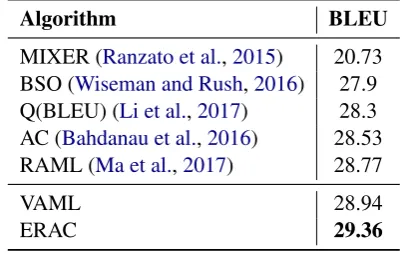
Based on the setting, the comparison is summa-rized in Table2.8 As we can see, both VAML and ERAC outperform previous methods, with ERAC leading the comparison with a significant margin. This further verifies the effectiveness of the two proposed algorithms.
Algorithm BLEU
MIXER (Ranzato et al.,2015) 20.73 BSO (Wiseman and Rush,2016) 27.9 Q(BLEU) (Li et al.,2017) 28.3 AC (Bahdanau et al.,2016) 28.53 RAML (Ma et al.,2017) 28.77
VAML 28.94
ERAC 29.36
Table 2: Comparison with existing algorithms on IWSTL 2014 dataset for MT. All numbers of pre-vious algorithms are from the original work.
6.4 Ablation Study
Due to the overall excellence of ERAC, we study the importance of various components of it, hope-fully offering a practical guide for readers. As the input feeding technique largely slows down the training, we conduct the ablation based on the model variantwithoutinput feeding.
Firstly, we study the importance of two tech-niques aimed for training stability, namely the tar-get network and the smoothing technique (§4.2). Based on the MT task, we vary the update speedβ
of the target critic, and theλvar, which controls the
8For a more detailed comparison of performance together
with the model architectures, see Table7in AppendixC.
H H
H H
HH
λvar
β
0.001 0.01 0.1 1
0 27.91 26.27† 28.88 27.38† 0.001 29.41 29.26 29.32 27.44
Table 3: Average validation BLEU of ERAC. As a reference, the average BLEU is 28.1 for MLE. λvar= 0means not using the smoothing technique.
β = 1means not using a target network. †
indi-cates excluding extreme values due to divergence.
strength of the smoothness regularization. The av-eragevalidation performances of different hyper-parameter values are summarized in Tab.3.
• Comparing the two rows of Tab. 3, the smooth-ing technique consistently leads to performance improvement across all values ofτ. In fact, re-moving the smoothing objective often causes the training to diverge, especially when β = 0.01 and1. But interestingly, we find the di-vergence does not happen if we update the tar-get network a little bit faster (β = 0.1) or quite slowly (β = 0.001).
• In addition, even with the smoothing technique, the target network is still necessary. When the target network is not used (β = 1), the perfor-mance drops below the MLE baseline. How-ever, as long as a target network is employed to ensure the training stability, the specific choice of target network update rate does not matter as much. Empirically, it seems using a slower (β= 0.001) update rate yields the best result.
en-0.000 0.005 0.010 0.020 0.045 26.0
27.0 28.0 29.0 30.0
BLEU
Dev Test
(a) Machine translation
0.000 0.001 0.005 0.010 0.020 29.5
30.0 30.5 31.0 31.5
BLEU
Dev Test
[image:9.595.105.498.64.219.2](b) Image captioning
Figure 1: ERAC’s average performance over multiple runs on two tasks when varyingτ.
tropy regularization can easily cause the actor to diverge. Specifically, the model diverges whenτ
reaches0.03on the image captioning task or0.06 on the machine translation task. On the other hand, as we decreaseτ from the best value to 0, the per-formance monotonically decreases as well. This observation further verifies the effectiveness of en-tropy regularization in ERAC, which well matches our theoretical analysis.
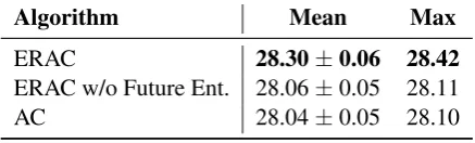
Finally, as discussed in§4.2, ERAC takes the ef-fect of future entropy into consideration, and thus is different from simply adding an entropy term to the standard policy gradient as in A3C (Mnih et al.,2016). To verify the importance of explicitly modeling the entropy from future steps, we com-pared ERAC with the variant that only applies the entropy regularization to the actor but not to the critic. In other words, theτ is set to 0 when per-forming policy evaluating according to Eqn. (4.2), while the τ for the entropy gradient in Eqn. (20) remains. The comparison result based on 9 runs on test set of IWSTL 2014 is shown in Table4. As we can see, simply adding a local entropy gradient does not even improve upon the AC. This further verifies the difference between ERAC and A3C, and shows the importance of taking future entropy into consideration.
Algorithm Mean Max
ERAC 28.30±0.06 28.42
ERAC w/o Future Ent. 28.06±0.05 28.11
AC 28.04±0.05 28.10
Table 4: Comparing ERAC with the variant with-out considering future entropy.
7 Discussion
In this work, motivated by the intriguing con-nection between the token-level RAML and the entropy-regularized RL, we propose two algo-rithms for neural sequence prediction. Despite the distinct training procedures, both algorithms com-bine the idea of fine-grained credit assignment and the entropy regularization, leading to positive em-pirical results.
However, many problems remain widely open. In particular, the oracle Q-functionQφwe obtain
[image:9.595.72.291.645.711.2]References
Dzmitry Bahdanau, Philemon Brakel, Kelvin Xu, Anirudh Goyal, Ryan Lowe, Joelle Pineau, Aaron Courville, and Yoshua Bengio. 2016. An actor-critic algorithm for sequence prediction. arXiv preprint arXiv:1607.07086.
Dzmitry Bahdanau, Kyunghyun Cho, and Yoshua Ben-gio. 2014. Neural machine translation by jointly learning to align and translate. arXiv preprint arXiv:1409.0473.
Leemon Baird. 1995. Residual algorithms: Reinforce-ment learning with function approximation. In Ma-chine Learning Proceedings 1995, Elsevier, pages 30–37.
Samy Bengio, Oriol Vinyals, Navdeep Jaitly, and Noam Shazeer. 2015. Scheduled sampling for se-quence prediction with recurrent neural networks. InAdvances in Neural Information Processing Sys-tems. pages 1171–1179.
William Chan, Navdeep Jaitly, Quoc Le, and Oriol Vinyals. 2016. Listen, attend and spell: A neural network for large vocabulary conversational speech recognition. In Acoustics, Speech and Signal Pro-cessing (ICASSP), 2016 IEEE International Confer-ence on. IEEE, pages 4960–4964.
Hal Daum´e III and Daniel Marcu. 2005. Learning as search optimization: Approximate large margin methods for structured prediction. InProceedings of the 22nd international conference on Machine learning. ACM, pages 169–176.
Tuomas Haarnoja, Haoran Tang, Pieter Abbeel, and Sergey Levine. 2017. Reinforcement learning with deep energy-based policies. arXiv preprint arXiv:1702.08165.
Tuomas Haarnoja, Aurick Zhou, Pieter Abbeel, and Sergey Levine. 2018. Soft actor-critic: Off-policy maximum entropy deep reinforcement learning with a stochastic actor. arXiv preprint arXiv:1801.01290 .
Kaiming He, Xiangyu Zhang, Shaoqing Ren, and Jian Sun. 2016. Deep residual learning for image recog-nition. In Proceedings of the IEEE conference on computer vision and pattern recognition. pages 770– 778.
Sepp Hochreiter and J¨urgen Schmidhuber. 1997. Long short-term memory. Neural computation 9(8):1735–1780.
Po-Sen Huang, Chong Wang, Dengyong Zhou, and Li Deng. 2017. Toward neural phrasebased machine translation .
Andrej Karpathy and Li Fei-Fei. 2015. Deep visual-semantic alignments for generating image descrip-tions. In Proceedings of the IEEE conference on computer vision and pattern recognition. pages 3128–3137.
Alex M Lamb, Anirudh Goyal ALIAS PARTH GOYAL, Ying Zhang, Saizheng Zhang, Aaron C Courville, and Yoshua Bengio. 2016. Professor forcing: A new algorithm for training recurrent net-works. InAdvances In Neural Information Process-ing Systems. pages 4601–4609.
Jiwei Li, Will Monroe, and Dan Jurafsky. 2017. Learn-ing to decode for future success. arXiv preprint arXiv:1701.06549.
Timothy P Lillicrap, Jonathan J Hunt, Alexander Pritzel, Nicolas Heess, Tom Erez, Yuval Tassa, David Silver, and Daan Wierstra. 2015. Continu-ous control with deep reinforcement learning. arXiv preprint arXiv:1509.02971.
Tsung-Yi Lin, Michael Maire, Serge Belongie, James Hays, Pietro Perona, Deva Ramanan, Piotr Doll´ar, and C Lawrence Zitnick. 2014. Microsoft coco: Common objects in context. In European confer-ence on computer vision. Springer, pages 740–755.
Minh-Thang Luong, Hieu Pham, and Christopher D Manning. 2015. Effective approaches to attention-based neural machine translation. arXiv preprint arXiv:1508.04025.
Xuezhe Ma, Pengcheng Yin, Jingzhou Liu, Graham Neubig, and Eduard Hovy. 2017. Softmax q-distribution estimation for structured prediction: A theoretical interpretation for raml. arXiv preprint arXiv:1705.07136.
Cettolo Mauro, Girardi Christian, and Federico Mar-cello. 2012. Wit3: Web inventory of transcribed and translated talks. InConference of European Associ-ation for Machine TranslAssoci-ation. pages 261–268.
Volodymyr Mnih, Adria Puigdomenech Badia, Mehdi Mirza, Alex Graves, Timothy Lillicrap, Tim Harley, David Silver, and Koray Kavukcuoglu. 2016. Asyn-chronous methods for deep reinforcement learning. In International Conference on Machine Learning. pages 1928–1937.
Volodymyr Mnih, Koray Kavukcuoglu, David Silver, Andrei A Rusu, Joel Veness, Marc G Bellemare, Alex Graves, Martin Riedmiller, Andreas K Fidje-land, Georg Ostrovski, et al. 2015. Human-level control through deep reinforcement learning. Na-ture518(7540):529.
Ofir Nachum, Mohammad Norouzi, Kelvin Xu, and Dale Schuurmans. 2017. Bridging the gap between value and policy based reinforcement learning. In Advances in Neural Information Processing Sys-tems. pages 2772–2782.
Kishore Papineni, Salim Roukos, Todd Ward, and Wei-Jing Zhu. 2002. Bleu: a method for automatic eval-uation of machine translation. In Proceedings of the 40th annual meeting on association for compu-tational linguistics. Association for Computational Linguistics, pages 311–318.
Marc’Aurelio Ranzato, Sumit Chopra, Michael Auli, and Wojciech Zaremba. 2015. Sequence level train-ing with recurrent neural networks. arXiv preprint arXiv:1511.06732.
Steven J Rennie, Etienne Marcheret, Youssef Mroueh, Jarret Ross, and Vaibhava Goel. 2016. Self-critical sequence training for image captioning. arXiv preprint arXiv:1612.00563.
Alexander M Rush, Sumit Chopra, and Jason We-ston. 2015. A neural attention model for ab-stractive sentence summarization. arXiv preprint arXiv:1509.00685.
John Schulman, Pieter Abbeel, and Xi Chen. 2017. Equivalence between policy gradients and soft q-learning.arXiv preprint arXiv:1704.06440.
Shiqi Shen, Yong Cheng, Zhongjun He, Wei He, Hua Wu, Maosong Sun, and Yang Liu. 2015. Minimum risk training for neural machine translation. arXiv preprint arXiv:1512.02433.
Ilya Sutskever, Oriol Vinyals, and Quoc V Le. 2014. Sequence to sequence learning with neural net-works. InAdvances in neural information process-ing systems. pages 3104–3112.
Oriol Vinyals, Alexander Toshev, Samy Bengio, and Dumitru Erhan. 2015. Show and tell: A neural im-age caption generator. InComputer Vision and Pat-tern Recognition (CVPR), 2015 IEEE Conference on. IEEE, pages 3156–3164.
Ronald J Williams and Jing Peng. 1991. Function opti-mization using connectionist reinforcement learning algorithms.Connection Science3(3):241–268.
Sam Wiseman and Alexander M Rush. 2016. Sequence-to-sequence learning as beam-search op-timization. arXiv preprint arXiv:1606.02960.
Kelvin Xu, Jimmy Ba, Ryan Kiros, Kyunghyun Cho, Aaron Courville, Ruslan Salakhudinov, Rich Zemel, and Yoshua Bengio. 2015. Show, attend and tell: Neural image caption generation with visual at-tention. In International Conference on Machine Learning. pages 2048–2057.
Brian D Ziebart. 2010. Modeling purposeful adaptive behavior with the principle of maximum causal en-tropy. Carnegie Mellon University.