Creep Modelling of a Material by Non Linear Modified Schapery’s Viscoelastic Model

(1)

http://www.scirp.org/journal/wjet ISSN Online: 2331-4249 ISSN Print: 2331-4222

DOI: 10.4236/wjet.2017.54063 Nov. 30, 2017 754 World Journal of Engineering and Technology

Creep Modelling of a Material by Non-Linear

Modified Schapery’s Viscoelastic Model

Priska Kuida Atchounga, Grégoire Kamdjo, Emmanuel Foadieng, Pierre Kisito Talla

Laboratory of Mechanics and Modelling of Physical Systems (L2MSP), Department of Physics, University of Dschang, Dschang, Cameroon

Abstract

This research work aims at modeling the creep behavior of a material by a non-linear schapery’s viscoelastic model. We started with analytical part where three powerful methods of creep modeling have been developed and compared. That is the Heaviside, the Nordin and Varna and lastly our own proposed methods. From this preliminary study, it came out that our method is different to the two others because we took into account the loading time at the creep beginning. Besides we studied several loading programs and re-tained a five order non-linear polynomial which is the program that gave us satisfactory results. The other loading functions led to divergent results and wasn’t present here as consequence. In the second part of this work, we de-voted ourselves to the determination of non-linear parameters in the scha-pery’s viscoelasticity equation, through a well developed and illustrated me-thodology. From this study, it is straight forward that non-linear parameters are stress dependent; confirming the results of several authors that preceded us in this studying field.

Keywords

Non-Linear Viscoelasticity, Creep, Strain, Stress, Schapery

1. Introduction

Creep is a physical phenomenon affecting many materials like woods, iron etc. in engineering structures like buildings. Before choosing a given material in en-gineering works, one must know very well its creep behavior in order to appre-ciate the lifespan of the structure. In such structures a deformation occurs when a material undergoes certain load. When it comes to study this phenomenon in the laboratory, we usually choose a normalized test material and with the help of

How to cite this paper: Atchounga, P.K., Kamdjo, G., Foadieng, E. and Talla, P.K. (2017) Creep Modelling of a Material by Non-Linear Modified Schapery’s Viscoelas-tic Model. World Journal of Engineering and Technology, 5, 754-764.

https://doi.org/10.4236/wjet.2017.54063

Received: September 1, 2017 Accepted: November 26, 2017 Published: November 30, 2017

http://creativecommons.org/licenses/by/4.0/

(2)

DOI: 10.4236/wjet.2017.54063 755 World Journal of Engineering and Technology

a test machine we submit this material to a certain stress and follow back the deformation that occurs over the time. The ability to carry out reliable creep tests in a reasonable time at low stress levels allows a designer to have much more confidence in the data for creep-rupture behavior for materials and allows confident prediction of structural lifetimes. The inconvenience of this experi-mental method is that it can’t permit to follow the behavior of a material over a large period of time, so it is limited. In order to solve this problem, it is necessary to develop theoretical methods that can allow to model and to predict the creep behavior over a very large period of time in terms of years or even century.

Many authors [1] [2] [3] [4] [5] devoted their works to the creep modeling through experimental and theoretical methods. In this paper, we develop a theoretical method from the well known schapery’s equation for viscoelasticity. The main task consists of determining the non-linear parameters. We started by presenting the method where the loading and the unloading of the material are described by Heaviside step function. Because this method presents shortcom-ings [6], it has been followed by the Nordin and Varna method and completed lastly by our analytical method.

2. Non-Linear Viscoelastic Material Model

The non-linear viscoelastic Schapery model [7] [8] is given by

( )

(

)

(

2

( ) ( )

)

0 0 1 ₀

d

d d

t g t

t g D t g D σ σ

ε σ σ σ ψ ψ τ

τ

′

= +

∫

∆ − (1)

where the reduced times are given by

( )

(

)

0

d

t t

aσ t

ψ

σ

′ =

′

∫

(2)

and

( )

(

)

0

dt

a t

τ

σ ψ

σ

′ ′ =

′

∫

(3)

where aσ is a shift factor. The parameters g0, g1, g2 and aσ are functions of strain.

D0 = D(0) is the initial value of creep compliance and ∆ =D D t

( )

−D0 is the

transient component of the creep compliance. When aσ =g0=g1=g2=1,

Eq-uation (1) reduces to

( )

0

( )

₀

(

) ( )

d d d

t t

t D t D t

σ

ε

σ

τ

= + ∆

∫

− ₍₄₎

Or

( )

₀

(

) ( )

d d d

t t

t D t

σ

ε

τ

=

∫

− ₍₅₎

(3)

( )

0 0

( )

0 1

( )

0 2

( )

0 1

a_σ =g =g =g = (6)

Many methods have been developed to determine the material parameters in Equation (1), see [6]-[11].

3. Methods of Analysis

3.1. Step-Stress Hypothesis

Under step-stress hypothesis, that is,

σ

( )

t =

σ

0H t

( )

, where H(t) is the

Heavi-side step function, Equation (1) takes the form

( )

(

)

(

2

( )

0 0

( )

)

0 0 0 0 1 0 ₀

d

d d

t g H

t g D g D σ σ τ

τ

′

= +

∫

∆ − (7)

( )

0

( )

0 0 0 1

( )

0 ₀

(

) ( )

2 0 0

( )

d

t

t g D g D g

ε = σ σ + σ

∫

∆ ψ ψ− ′ σ σ δ τ τ ₍₈₎

( )

0

( )

0 0 0 1

( ) ( )

0 2 0 0

( )

0

t

t g D g g D

aσ

ε σ σ σ σ σ

σ

 

= + ∆ _ _

  (9) where δ is the Dirac delta function. Equation (9) is the material response when the stress is applied by the Heaviside step function.

3.2. Method by Nordin and Varna

Let the stress be given by

( )

0

( )

(

)

1

2

t σ H t H t t

σ = _ + − _₍₁₀₎

Then

( )

0

( )

0

(

)

2 2 2 0 2 1

2 2

g σ =g _σ _H t +_g σ −g _σ __H t−t

     (11)

and

( ) ( )

0 0

( )

0

(

)

2 2 2 2 0 2 1

2 2 2

g

σ σ

t =

σ

_g _

σ

_H t +_ g

σ

−g _

σ

__H t−t _

    

  (12)

Differentiating Equation (12) with respect to time gives

( ) ( )

(

2

)

₀ ₀

( )

₀

(

)

2 2 2 0 2 1

2 2 2

g t

g t g g t t

t

σ σ σ σ _δ _σ σ _δ

∂ ₌    ₊ ₋   ₋ 

      

∂        (13)

Substituting Equation (13) in Equation (1) when t≥t1 gives

( )

(

)

( )

(

) (

)

0

0 0 0 0 1 0 0 2 ₀

0

1 0 0 2 0 2 ₀ 1

1 2 2 1 2 d 2 2 t t

t g D g g D

g g g D t t

σ

ε σ σ σ σ ψ ψ

σ

σ σ σ ψ ψ δ τ

  _′ = + _ _ ∆ −      _′ + _ − _ __ ∆ − −    

∫

(14)

After integrating with mathematical formulae Equation (14) yields

( )

(

)

( )

0 1 1

0 0 0 0 1 0 0 2

0 0

0 1

1 0 0 2 0 2

0

1

2 2 2

1

+ 2

2 2

t t t

t g D g g D

a a

t t

g g g D

a

σ σ

ε σ σ σ σ

σ σ

σ

σ σ σ

(4)

which represents the material response under a tress defined by Equation (10).

3.3. Proposed Method

We now consider case where the stress is given by

( )

1

0 1

, ,

f t t t

t t t

σ

 =  _≥   (16)

where f

( )

0 =0 and f t

( )

1 =

σ

0. Then the strain at time t≥t1 is given by

( )

1

(

)

(

2

( )

)

0 0 0 0 1 0 ₀

d

d d

t g

t g D g D σ σ

τ

′

= +

∫

∆ − ₍₁₇₎

where

( )

1 1 1 1 0 0 0 0 0 0

0 0 0 0

d d

d d d d

t

t t t

t t

a a

t t t t

a a a a

τ

σ σ

τ

σ σ σ σ

ψ ψ

σ σ

σ σ σ σ

′ ′ ′ − = −   ′ ′ ′ ′ = + −_ + _  

∫

(18)

( )

10 1

( )

0

d

t

t t t

a_σ τ a_σ

ψ ψ

σ σ

′ −

′

− = +

∫

₍₁₉₎

By combining Equation (19) and Equation (17), we have

( )

1

(

( )

)

(

( )

)

( )

)

0 0 0 0

2 1

1 0 1

0

d d

d

t

t g D

g

t t t

g t D

a_σ τ a_σ t

ε σ σ

σ τ σ τ σ

σ σ τ

=  ₋ _′  + ∆ _ + _ ′ 

∫

 (20)

Using midpoint rule, which is third-order accurate with respect to t1 [12], and

with τ = t1/2 then it follows that

( )

(

)

(

( )

)

(

)

1 1 1 1 1 2 1 1 1 1 1 1 2 d d 2 2 2 2 3 3 4 4 t t t t t t t

a t a t t t

a

t t

a a f

τ

σ σ

σ

σ σ

σ σ _σ

σ − ′ ′ = = ′ ′   +     _ _   = =            _ _  _ _    

∫

(21)

If the ramp loading is approximated to be linear, then f

(

3t1 4

)

=3

σ

0 4. So

we have

( )

(

)

(

)

1 1 0 2 d 3 4

t t t

a

a t

τ

σ

σ σ σ

′ = ′

∫

(22)

Let us apply second-order [13] accurate numerical differentiation formula to the function in Equation (20), it comes that

( )

(

)

( )

(

)

(

( )

)

( )

(

( )

)

( )

1

2 2 1 1 2 2 0 0

1 1

2

d 0 0

d

t

g g t t g g

t t

τ

σ τ σ τ σ σ σ σ σ σ

τ

=

  ₋

  ≈ =

 

  (23)

(5)

Equa-DOI: 10.4236/wjet.2017.54063 758 World Journal of Engineering and Technology

tion (16) is

( )

0

( )

0 0 0 1

( ) ( )

0 2 0 0

( )

0

t

t g D g g D

a_σ

ε σ σ σ σ σ

σ

 

= + ∆ _ + Ω_

  (24) where

(

)

( )

1

0 0

1 1

2 3 4

t

aσ σ aσ σ

 

Ω = _ − _

  (25) Only a rather moderate modification is made in the proposed method as compared to the step loading case, where Ω = 0. Furthermore, in linear case the proposed correction method yields

( )

1

0

2

t

t D t

ε

=

σ

_ − _

  (26)

which is the Zapas-Phillips [11] [14] correction method for linear viscoelastic systems.

4. Numerical Studies

In the following subsections we compare the accuracy of the Heaviside step loading, Nordin-Varna and the proposed method.

4.1. Linear Case

In linear case non-linear parameters in Equation (1) equals to one. Then the Nordin-Varna method for the creep formulation at time t ≥ t1 is given by

( )

0

( )

0

(

)

0 0 1

2 2

t D σ D t σ D t t

ε = σ + ∆ + ∆ − ₍₂₇₎

( )

0

( )

(

)

1

2

t σ D t D t t

ε = _ + − _ (28)

and with the proposed method it is given by

( )

1 1

0 0 0 0

2 2

t t

t D D t D t

ε

=

σ

+ ∆

σ

_ − _=

σ

_ − _

    (29)

The exact value for the strain at time t ≥ t1 is

( )

1

(

) ( )

0 d

t

t D t

ε =

∫

−τ σ τ τ (30)

If the loading is carried out with a constant stress rate, then

( )

1

(

)

0 d

t

t D t

ε =σ

∫

−τ τ (31)

where σ σ= 0 t1. Now it can be seen that by applying numerical integration

rule, to Equation (31) we get the Nordin-Varna method and by applying mid-point rule we get the proposed method, respectively. Error estimate for the tra-pezoidal rule is [13]

3 1

12 t

(6)

and for the midpoint rule [13] 3 1

24 t

e= D′′ (33)

To summarize, in linear case error in the proposed method is half of error in the Nordin-Varna method.

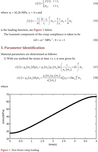
4.2. Non-Linear Case, Creep Test with Non-Linear Ramp

The creep test that we study has the following form

( )

1

0 1

, ,

f t t t

t

t t

ε

σ



=  _≥





(34)

where σ0 = 42.26 MPa, t1 = 4 s and

( )

5 1

0 0 0

1 1

2

1 3 1

6 2 4

t t t

f t

t σ t σ σ

 − 

= − _ _ + +

  (35)

is the loading function, see Figure 1 below.

The transient component of the creep compliance is taken to be 1

MPa , 0 1

n

D αt − n

∆ =   (36)

5. Parameter Identification

Material parameters are determined as follows:

1) With our method the strain at time t ≥ t1 is now given by

( )

0

( )

0 0 0 1

( ) ( )

0 2 0

( )

0 0

n t

t g D g g

a_σ

ε

σ

σ α

σ

 

= + _ + Ω_

  (37)

( )

1

( ) ( )

0

( )

2 0

[

]

0 0 0 0 0

0

n n

g g

t g D a t a

aσ σ σ

σ σ

ε σ σ α σ

σ

= + + Ω ₍₃₈₎

[image:6.595.204.538.206.723.2]

where

Figure 1. Non-linear ramp loading.

0 0.5 1 1.5 2 2.5 3 3.5 4

10 20 30 40 50 60 70

time(s)

s

tr

e

s

(M

P

a

(7)

(

)

( )

1

0 0

1 1

2 3 4

t

a_σ σ a_σ σ

 

Ω =  − 

 

  (39) 2) Creep test data with different constant stress levels is fitted to

( )

0

( )

0

n

f t = +A B a_ _σ

σ

t+ Ωa_σ

σ

_ (40)

where

( )

( ) ( )

( )

0

0 0 0

1 0 2 0

0

n

f t t

A g D

g g B aσ ε σ σ σ σ α σ =   =    =   (41)

3) Now the values of A(σ0) and B(σ0) are known for all constant stress levels.

4) Parameter A is fitted to some proper function A(σ). We have used five or-der polynomial to approximate A(σ), in this study. Then the parameter D0 can

be determined using initial condition A

( )

0 =g0

( )

0 D0 =D0. Since

( )

0 0

g

σ

=A

σ

D the parameter g₀ can be also determined [15].

5) Parameter B is fitted to some proper function B(σ). In this study, we have used five order polynomial to approximate B(σ). Then the parameter α can be determined using initial condition

( )

1

( ) ( )

0

( )

2 0

0 0 n g g B aσ α α = = _.

6) We have 1

( ) ( )

0

( )

2 0

( )

0 0

g g B

a_σ

σ σ σ

σ = α . The value of B(σ0)/α is known for all

constant stress levels, this value is denoted C. Parameter C is fitted to some proper function C [16]. We have used five order polynomial to approximate C(σ). Then, parameters g1, g2 and aσ can be determined using initial conditions

( )

1 0 2 0 0 1

g =g =a_σ = .

7) Since

( )

1

( ) ( )

0

( )

0 0 0

0

n g g

a B σ σ σ σ α σ

= then we have

( ) ( )

(

)

(

( )

)

(

)

( )

(

)

1 0 2 0 0

0

ln

g g B

n

a_σ

σ

α σ

σ

=

The preceding methodology leads us to the following values:

6 1 6 1

0 160 10 MPa ; 1.03 10 MPa and 0.24

D = × − −

α

= × − − n= (42)

Simulated non-linear parameters are

( )

7 5 5 4 3 3 2

0

8 5 5 4 4 3 2 2

1

7 5 5 4 3 3 2

2

7 5 5 4 3 3

3.2 10 5.7 10 3.9 10 0.13 2 11

8.5 10 1.3 10 8.1 10 2.4 10 0.34 0.83

4.9 10 8.5 10 5.7 10 0.19 2.9 17

5.7 10 9.7 10 6.4 10 0.21

g g g a_σ

σ σ σ σ σ σ

σ σ σ σ σ

− − − − − − − − − − − − − = × − × + × − + − = × − × + × − × + − = × − × + × − + −

= × − × + × − 2

3.2σ 18

      ₊ ₋  (43)

6. Relative Errors and Creep Curves

(8)

( )

t

( )

t

e t

t

ε ε

ε

−

= (44)

where

ε

( )

t the true value of the strain in the creep test and

ε

( )

t is the

nu-merically approximated value of strain. The Table 1 below depicts relative er-rors:

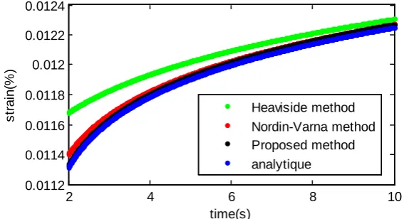
Error estimates shows that the proposed method produces the smallest error. The computed strain in creep test with different methods is shown in Figure 2 below.

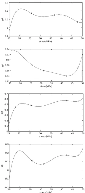
Non-linear parameters are shown in Figure 3.

Figure 3 depicts the predicted non-linear parameters (straight curve) with our proposed method and the true value of non-linear parameters (disconti- nuous curve with “+” sign). From these figures it is evident that the simulated non-linear parameters are in good agreement with the true value of the non-linear parameters. We can notice from our results that stress highly influences the value of material non-linear parameters; which is a confirmation that parameters

g0, g1, g2 and aσ in the Schapery’s viscoelasticity equation are stress dependent [7]

[image:8.595.230.514.455.609.2]

[8]. These results are matching perfectly with those obtained by [1] [2] [3] [4] when they were dealing with physical and mechanical properties of some Ca-meroonians woods. Authors [17] [18] [19] when dealing with non-linear creep and relaxation obtained similar results in their scientific works.

Figure 2 is just depicting the advantage of predicting creep behavior of ma-terial with our method. It is clear that the predicted creep curve is so close to the true value of the creep to be distinguished. The lower value of the relative esti-mating errors is just reinforcing the method.

[image:8.595.207.542.661.728.2]

Figure 2. Strain as a function of time in creep test.

Table 1. Relative errors in creep test.

Method Error (%)

Heaviside step loading 0.01

Nordin-Varna 0.0028

Proposed 0.0016

2 4 6 8 10

0.0112 0.0114 0.0116 0.0118 0.012 0.0122 0.0124

time(s)

s

tra

in

(%

)

(9)

[image:9.595.232.513.68.702.2]

DOI: 10.4236/wjet.2017.54063 762 World Journal of Engineering and Technology Figure 3. Non-linear parameters as a function of stress.

15 20 25 30 35 40 45 50

0.9 1 1.1 1.2 1.3

stress(MPa)

g0

15 20 25 30 35 40 45 50

0.82 0.84 0.86 0.88 0.9 0.92 0.94

stress(MPa)

g1

15 20 25 30 35 40 45 50

0 0.1 0.2 0.3 0.4 0.5 0.6 0.7

stress(MPa)

g2

15 20 25 30 35 40 45 50

-0.2 -0.1 0 0.1 0.2 0.3

stress(MPa)

(10)

7. Conclusion

We have presented in this paper a powerful method which takes in to account the finite ramp time in the Schapery’s non-linear viscoelastic equation. It came out that the method is a good predicting tool of strain in creep test, because it is doing while minimizing the relative error. At the end material non-linearity pa-rameters that have been simulated from the proposed method are in good agreement with those found in literature. The authors [20], [21] and [16] applied different processes in their works to predict long term creep of composites and they came out with good results. In the future we can see how to apply our cor-rection method to what they did in order to have different point of view.

References

[1] Talla, P.K., Foadieng, E., Fouotsa, W.C.M., Fogue, M., Bishweka, S., Ngarguededjim K.E., Alabeweh, F.S. and Foudjet, A. (2015) A Contribution to the Study of Entan-drophragma Cylindricum Sprague and Lovoa Trichilioides Harms Long Term be-haviour. Revue scientifique et Technique Forêt et Environnement du Bassin du Congo, X, 10-21.

[2] Talla, P.K., Mabekou, J.S., Fogue, M., Fomethe, A., Bawe, G.N., Foadieng, E. and Foudjet, A. (2010) Non-Linear Creep Behavior of Raphia vinifera L. Arecacea under Flexural Load. International Journal of Mechanics and Solids, 5, 151-172.

[3] Talla, P.K. (2008) Contribution à l’analyse mécanique de Raphia vinifera L. Arecacea. Thèse de Doctorat (Ph.D), Université de Dschang, Faculté des Sciences, Cameroun.

[4] Talla, P.K., Pelab, F.B., Fogue, M., Fomethe, A., Bawe, G.N., Foadieng, E. and Foudjet, A. (2007) Non-Linear Creep Behavior of Raphia vinifera L. Arecacea. In-ternational Journal of Mechanics and Solids, 2, 1-11.

[5] Foadieng, E., Fogue, M. and Talla, P.K. (2012) Effect of the Span Length on the Deflection and the Creep Behavior of Raffia Bamboo Vinifera L. Arecacea Beam.

International Journal of Material Science, 7, 153-167.

[6] Nordin, L.O. and Varna, J. (2006) Methodology for Parameter Identification in Non-Linear Viscoelastic Material Model. Mech. Time Matter, 9, 259-280.

[7] Schapery, R.A. (1969) On the Characterization of Non-Linear Viscoelastic Mate-rials. Polymer Engineering & Science, 9, 295-310.

https://doi.org/10.1002/pen.760090410

[8] Lou, Y.C. and Schapery, R.A. (1971) Viscoelastic Characterization of a Non-Linear Fiber-Reinforced Plastic. Journal of Composite Materials, 5, 208-234.

https://doi.org/10.1177/002199837100500206

[9] Kshitish, A.P. (2009) Linear and Non-Linear Viscoelastic Characterization of Pro-ton Exchange Membranes and Stress Modeling for Fuel Cell Application. Doctor of Philosophy thesis, Virginia Polytechnic Institute and State University, USA. [10] Chien, W.H., Rashid, K.A., Eyad, A.M., Dallas, N.L. and Gordon, D.A. (2011)

Nu-merical Implementation and Validation of a Non-Linear Viscoelastic and Viscop-lastic Model for Asphalt Mixes. International Journal of Pavement Engineering, 12, 433-447.https://doi.org/10.1080/10298436.2011.574137

[11] Zapas, L.J. and Philips, J.C. (1971) Simple Shearing Flows in Polyisobutylene Solu-tions.Journal of Research of the National Bureau of Standards, 75A, 33-41.

(11)

DOI: 10.4236/wjet.2017.54063 764 World Journal of Engineering and Technology [12] Bakhvalov, N.S. (1977) Numerical Methods: Analysis, Algebra, Ordinary

Differen-tial Equations. MIR, Moscow.

[13] Rami, M.H.K. and Anastasia, H.M. (2003) Numerical Finite Element Formulation of the Schapery Non-Linear Viscoelastic Material Model. International Journal for Numerical Methods in Engineering, 59, 25-45.

[14] Ahlberg, J.H., Nilson, E.N. and Walsh, J.L. (1967) The Theory of Splines and Their Applications. Academic Press, New York.

[15] Benjamin, B. (2013) Interpolation Polynomiale. Agrégation de mathématiques, Op-tion modélisaOp-tion, Université de Rennes 1.

[16] Ratchada, S. and Raffaella, D.V. (2011) A Mathematical Model for Creep, Relaxa-tion and Strain Stiffening in Parallel-Fibered Collagenous Tissues. Journal of Medi-cal Engineering and Physics, 33, 1056-1063.

https://doi.org/10.1016/j.medengphy.2011.04.012

[17] Calgcagno, B., Lopez, G.M., Kuhns, M. and Lakes, R.S. (2008) On the Non-Linear Creep and Recovery of Open Cell Earplug Foams. Journal of Cellular Polymers, 27, 165-178.

[18] Kaouther, B.A.A. (2010) Relations entre propriétés rhéologiques et structure mi-croscopique de dispersions de particules d’argile dans des solutions de polymères. Thèse de Doctorat (Ph.D.), Université de Haute Alsace, France.

[19] Ashish, O., Ray, V.J. and Roderic, S.L. (2003) Interralation of Creep and Relaxation for Non-Linearly Viscoelastic Materials: Application to Ligament and Metal. Rheo-logica Acta, 42, 557-568.https://doi.org/10.1007/s00397-003-0312-0

[20] Tuttle, M.E. and Brinson, H.F. (1985) Prediction of the Long-Term Creep Com-pliance of General Composite Laminates. Experimental Mechanics,26, 89-102. https://doi.org/10.1007/BF02319961

http://www.scirp.org/journal/wjet

: 10.4236/wjet.2017.54063

http://creativecommons.org/licenses/by/4.0/

https://doi.org/10.1002/pen.760090410

https://doi.org/10.1177/002199837100500206

7.

https://doi.org/10.6028/jres.075A.005

https://doi.org/10.1016/j.medengphy.2011.04.012

https://doi.org/10.1007/s00397-003-0312-0

https://doi.org/10.1007/BF02319961