Original citation:
Zhou, Shuyu, Zhang, Xiandong, Chen, Bo and Velde, Steef van de. (2014) Tactical fixed job scheduling with spread-time constraints. Computers And Operations Research , Volume 47 . pp. 53-60.
Permanent WRAP url:
http://wrap.warwick.ac.uk/59360
Copyright and reuse:
The Warwick Research Archive Portal (WRAP) makes this work of researchers of the University of Warwick available open access under the following conditions. Copyright © and all moral rights to the version of the paper presented here belong to the individual author(s) and/or other copyright owners. To the extent reasonable and practicable the material made available in WRAP has been checked for eligibility before being made available.
Copies of full items can be used for personal research or study, educational, or not-for-profit purposes without prior permission or charge. Provided that the authors, title and full bibliographic details are credited, a hyperlink and/or URL is given for the original metadata page and the content is not changed in any way.
Publisher’s statement:
NOTICE: this is the author’s version of a work that was accepted for publication in Computers And Operations Research. Changes resulting from the publishing process, such as peer review, editing, corrections, structural formatting, and other quality control mechanisms may not be reflected in this document. Changes may have been made to this work since it was submitted for publication. A definitive version was subsequently published Computers And Operations Research , Volume 47 . pp. 53-60.
http://dx.doi.org/10.1016/j.cor.2014.02.001 A note on versions:
The version presented here may differ from the published version or, version of record, if you wish to cite this item you are advised to consult the publisher’s version. Please see the ‘permanent WRAP url’ above for details on accessing the published version and note that access may require a subscription.
Tactical Fixed Job Scheduling
with Spread-Time Constraints
Shuyu Zhoua,b, Xiandong Zhangc, Bo Chend, Steef van de Veldeb
aDepartment of Mathematics, East China University of Science and Technology,
Shanghai 200237, China
bRotterdam School of Management, Erasmus University,
3000 DR Rotterdam, The Netherlands cSchool of Management, Fudan University,
Shanghai 200433, China
dWarwick Business School, University of Warwick,
Coventry CV4 7AL, UK
Abstract
We address the tactical fixed job scheduling problem with spread-time con-straints. In such a problem, there are a fixed number of classes of machines and a fixed number of groups of jobs. Jobs of the same group can only be processed by machines of a given set of classes. All jobs have their fixed start and end times. Each machine is associated with a cost according to its machine class. Machines have spread-time constraints, with which each ma-chine is only available forLconsecutive time units from the start time of the earliest job assigned to it. The objective is to minimize the total cost of the machines used to process all the jobs. For this strongly NP-hard problem, we develop a branch-and-price algorithm, which solves instances with up to 300 jobs, as compared with CPLEX, which cannot solve instances of 100 jobs. We further investigate the influence of machine flexibility by computational experiments. Our results show that limited machine flexibility is sufficient in most situations.
Keywords: machine scheduling, spread-time constraint, flexible manufacturing, branch and price, neighborhood search
1. Introduction
by Dantzig and Fulkerson [1]. In such a problem, there are a set J =
{J1, . . . , Jn}of n jobs and each job Jj (1≤j ≤n) requires processing
with-out interruption from a given start time rj to a given end time dj. Each
machine, while available all the time, can process at most one job at a time. The objective is to determine the minimum number of identical machines needed to process all the jobs. Gupta et al. [2] give an O(nlogn) time exact algorithm and they show that such a running time is the best possible.
In many production environments, jobs are classified into disjoint groups and machines into different classes. A machine of a specific class can only process jobs of some specific groups. In particular, a single-purpose machine is inflexible and can only process jobs of a specific group. Added with these constraints, the FJS problem becomes difficult. There are two main variants of such a general FJS problem: operational and tactical.
In the operational FJS problem, a fixed number of identical machines are given. One is to select a subset of jobs from J to process so as to maxi-mize the total profit from processing these jobs, where a profit is generated from processing a job. The problem has its roots on the capacity planning of aircraft maintenance personnel for KLM Royal Dutch Airlines (Kroon et al. [3], Kroon [4]), where each arriving plane requires one or more maintenance jobs, each within a fixed time period, and each available engineer is licensed to carry out jobs on at most two different aircraft types. Each maintenance job has a priority index. The objective is to find an assignment of aircraft to engineers so as to maximize the total priority index of all assigned main-tenance jobs. Kroon et al. [3] provide an exact algorithm when there is only one single machine class and two approximation algorithms when there are multiple machine classes. Eliiyi and Azizoglu [5], Bekki and Azizoglu [6], Eliiyi and Azizoglu [7], Solyali and Ozpeynirci [8], and Eliiyi and Az-izoglu [9] study the problem with various job characteristics and machine environments, such as spread-time constraints (see below for more details), working-time constraints, machine-dependent job weights, uniform parallel machines, etc.
The tactical FJS problem is a dual to its operational counterpart stated above, in which one is to minimize the total cost of processing all jobs of
serve all incoming aircraft on time with minimum total number of gates. If the number c of machine classes is fixed and c > 2, Kolen and Kroon [11] prove that the problem is strongly NP-hard. On the other hand, if c is not fixed, Kroon et al. [10] prove that the problem is strongly NP-hard even if preemption is allowed. They also present an exact branch-and-bound algorithm for solving the problem to optimality.
For a general overview of research in interval scheduling, we refer the reader to Kovalyov et al. [12] and Kolen et al. [13].
In many practical applications of the FJS model, the spread-time con-straints are also important, with which each machine is available only for L consecutive time units from the start of the earliest job assigned to it. Such constraints first appeared in the bus driver scheduling problem studied by Martello and Toth [14]. Fischetti et al. [15] show that the basic FJS problem with spread-time constraints is NP-hard and they develop an exact branch-and-bound algorithm. For the same problem, Fischetti et al. [16] provide a 2-approximation algorithm that runs in O(nlogn) time.
In this paper, we address the tactical (general) FJS problem with spread-time constraints (TFJSS). To the best of our knowledge, this study is the first to address the problem. Since the problem is strongly NP-hard, we provide a branch-and-price algorithm, which solves to optimality randomly generated instances with up to 300 jobs within one hour. Instances with 100 jobs are well solved to optimality within 40 seconds. This is in contrast to the fact that, on the standard ILP formulation of the problem, CPLEX cannot solve instances with 100 jobs within one hour. With the same algorithm, we solve the TFJSS problem with additional constraints.
branch-ing idea in solvbranch-ing the trainees schedulbranch-ing problem in a hospital department. Our computational experiments show that our design is efficient.
The paper is organized as follows. After providing two ILP formulations for the TFJSS problem in Section 2, one standard and the other for column generation purpose, we describe our branch-and-price algorithm in Section 3. Computational results of the algorithm are provided in Section 4, in which we test the computational effectiveness of our algorithm and, additionally, test a theory on machine flexibility as stated in Jordan and Graves [22]. We draw some conclusions in Section 5. In the appendix, we provide a neighborhood search algorithm that can be embedded in our branch-and-price algorithm to improve its efficiency in many cases.
2. Formulations
Denote by Mi the set of machines of class i (1 ≤ i ≤ c) and by Cj
(1≤j ≤n) the set of machine classes containing machines that can process job Jj. Let wi and Ji be, respectively, the cost of any machine of Mi and
the set of jobs that can be processed by a machine of Mi.
2.1. Basic formulation
Without loss of generality, we first re-index all jobs so that r1 ≤ r2 ≤
· · · ≤ rn. A pair of jobs Jj, Jk ∈ Ji with j < k are said to be compatible
with each other if they can be assigned together and processed by a single machine of Mi, i.e., r
k ≥dj and dk−rj ≤ L. For any Jj ∈ Ji (1≤ i≤ c),
let
Aj ={Jk ∈ Ji :k > j and jobJk is not compatible withJj}.
That is, Aj consists of all jobs having larger start times thanrj that cannot
be assigned to a machine together with job Jj due to either overlapping
processing intervals or the spread-time constraint. Define binary decision variable yi
k to represent whether or not machine
k ∈ Mi is used, and binary decision variable xijk to denote whether or not job Jj ∈ Ji is assigned to machine k ∈ Mi. The TFJSS problem can be
formulated as an ILP as follows:
z0 = min
c
∑
i=1 wi
∑
k∈Mi
subject to
xijk ≤yik, (Jj ∈ Ji, k∈Mi, i= 1, . . . , c) (2)
xijk+xiℓk ≤1, (Jℓ∈ Aj, Jj ∈ Ji, k∈Mi, i= 1, . . . , c) (3)
∑
i∈Cj
∑
k∈Mi
xijk = 1, (j = 1, . . . , n) (4)
xijk, yki ∈ {0,1}. (Jj ∈ Ji, k∈Mi, i= 1, . . . , c) (5)
The objective function (1) is to minimize the total cost of used machines. Constraints (2) guarantee that machine k is used when job Jj is assigned to
that machine. Constraints (3) make sure that the jobs are compatible on any used machine. Constraints (4) state that each job is processed exactly once. Finally, (5) are the binary constraints on the assignment variables.
2.2. Formulation for column generation
Define a single-machine schedule as a string of jobs that are compatible with each other. For any i = 1, . . . , c, let aijs be a binary constant that is equal to 1 if and only if jobJj ∈ Ji is a job in single-machine schedules.
Ac-cordingly, column ai
s = (ai1s, . . . , ains)T represents the jobs in single-machine
schedule s that can be processed by a machine of Mi. For convenience, in what follows, we often refer a single-machine schedule also as a column.
LetSi be the set of all single-machine schedules of jobs inJi. We
intro-duce binary decision variablesxis (s∈Si andi= 1, . . . , c) such thatxis= 1 if and only if single-machine schedule s is used for processing the correspond-ing jobs on a machine of Mi. Therefore, our problem is to select a set of
single-machine schedules so that all jobs in J are processed exactly once and the total machine cost is minimized. Consequently, the problem can be formulated in a form of column generation as follows:
zI = min c
∑
i=1
∑
s∈Si
wixis (6)
subject to
c
∑
i=1
∑
s∈Si
aijsxis≥1, j = 1, . . . , n, (7)
Constraints (7) ensure that each job is executed at least once. The reason why we use inequality rather than equality is to constrain the dual space and speed up the convergence. Note that the dual variables corresponding to constraint (7) are nonnegative. The binary constraints (8) ensure machine schedule s is selected once or not at all.
Since the number of columns involved in the above formulation can go exponential large with increased n, we apply column generation method. To this end, we relax the binary constraints on the variables to obtain the LP relaxation of ILP (6)–(8). Denote by XL an optimal solution of the LP
relaxation and by zL the corresponding optimal objective value.
3. The solution process
The column generation method solves the LP relaxation problem in which only a subset of the variables are available. An initial solution is generated by a greedy algorithm presented in Section 3.1. New columns will be added, which may decrease the solution value, if the optimal solution has not been determined yet. These new columns are identified through a pricing algo-rithm that solves an optimization problem at each iteration. We present the pricing algorithm in Section 3.2. To ensure that an integer solution is found, we apply a branch-and-price approach together with column generation. We present the details of the whole algorithm in Section 3.3.
3.1. Selection for initial solution
Our solution process starts with the following algorithm, which selects an initial solution.
Algorithm GR
Step 1. Re-index all jobs if necessary so thatr1 ≤r2 ≤ · · · ≤rn. Let S=∅
and j := 1.
Step 2. Ifj > n, then stop and output a feasible LP solutionX that corre-sponds to the set S of single-machine schedules (columns).
Step 3. Check whether there exists a single-machine schedule s ∈ S such that jobJj can be appended tosto form a valid single-machine schedule
s′. (a) If yes, set S := S\{s} ∪ {s′}; (b) if no, let ℓ = min{i : i∈ Cj} and construct a new single-machine schedule sℓ, which consists of the
single job Jj, and set S :=S ∪ {sℓ}; (c) in either case, set j := j+ 1
3.2. The pricing algorithm for column generation
According to the duality theory, a solution to a minimization LP problem is optimal if and only if thereduced cost of each variable is nonnegative. The reduced cost Psi of (relaxed) variablexis is given by
Psi =wi−
∑
Jj∈Ji λjaijs,
where λ1, . . . , λn are the values of the dual variables corresponding to the
current LP solution. To test whether the current solution is optimal, we determine if there exists a single-machine schedule s ∈ Si so that Pi
s is
negative. To this end, we solve the pricing problem of finding the machine schedule in Si with the minimum reduced cost for each i. Because wi is a
constant for any s∈Si, we essentially need to maximize
˜
Psi := ∑
Jj∈Ji
λjaijs. (9)
If the current value of ˜Pi
s ≤wi for each i, we have already found an optimal
solution for the LP relaxation problem. Otherwise, we use the following pricing algorithm to search for new columns {ais}to maximize (9).
The pricing algorithm is based on dynamic programming (DP) and uses a forward recursion that exploits the property that on each machine the jobs are sequenced in order of increasing indices. Furthermore, since our DP-based pricing algorithm will be combined with a branch-and-bound process and hence used iteratively, it is constrained to generate columns of those single-machine schedules in which each job Jj has a specified set Jj+ ⊆ J
of immediate successors, where an immediate successor of jobJj in a
single-machine schedule s is the job that is the first to be processed in s after completion of job Jj. Denote job precedence constraints by
P =
n
∪
j=1
J+
j . (10)
We refer the following DP-based algorithm as DP(P). For 1 ≤ j ≤ k ≤ n and 1≤i≤c, let
Fi(j, k) =
{
s ∈Si :Jj, Jk ∈ Ji are the first and last job in s
and
fi(j, k) =
{
maxs∈Fi(j,k)P˜si, if Fi(j, k)̸=∅
0, otherwise.
Then, after initialization fi(j, j) = λj for any Jj ∈ Ji (i = 1, . . . , c), the
recursion for k =j+ 1, . . . , n and Jk ∈ Ji is as follows:
fi(j, k) =
{
0, if Jk∈ Aj
maxℓ:j≤ℓ<k;J
k∈Jℓ+fi(j, ℓ) +λk, if Jk∈ Aj/ .
Let fi∗ = max1≤j≤k≤nfi(j, k) (i= 1, . . . , c).
Iffi∗ ≤wi for any i, then the current LP solution is optimal. Otherwise,
it is not and we need to introduce new columns to the problem. Candidates are associated with those ifor whichfi∗ > wi. An important implementation
issue is to determine the number of columns to add to the LP after having solved the pricing algorithm. The more columns we add per iteration, the fewer LPs we need to solve, but the bigger the LPs become. An empiri-cally good choice for our computational platform appears to be adding those ten columns that correspond to those ten values of i for which fi∗ are most positive. The pricing algorithm requires O(cn2) time and space.
We solve the LP problem after the addition of new columns and calculate the new set of dual variables λ1, . . . , λn. Then repeat the DP-based pricing
algorithm to test the optimality of our new LP solution. Such iteration pro-cess is repeated until we find an optimal LP solution to the original problem.
3.3. The branch-and-price algorithm
Recall that XL = {x˜is : s ∈ Si, i = 1, . . . , c} denote an optimal solution
of the LP relaxation problem of ILP (6)–(8). Throughout this subsection until the formal description of the branch-and-price algorithm at the end, we explain in detail how we deal withXL at the root node of our branching tree.
However, everything is applicable to the case where we are at any descendant node with replacement of XL by an optimal solution to the corresponding
LP problem at that node and “optimality” adjusted with respect to the corresponding sub-problem at the node.
If all the components {x˜is} of X
L are integers, then we find an optimal
this variable positive. Therefore, we use a different branching strategy, which is based on the notion of predecessors and successors.
For any given single-machine schedule s, all the jobs in s are processed in a unique sequence of increasing start times. Therefore, any job in s has a unique immediatepredecessor and successor, where we define the immediate predecessor (respectively, successor) of the first (respectively, last) job in s as a dummy jobJ0 (respectively, Jn+1). For any optimal LP solutionXL, let
Φ(XL) ={s:s ∈Si such that 0 <x˜is <1 for some 1≤i≤c}.
That is, Φ(XL) consists of those single-machine schedules (columns)
corre-sponding to fractional components of XL. Therefore, if XL is an integral
solution, then Φ(XL) =∅. Denote
Jf(XL) ={Jj ∈ J :Jj is a job ins ∈Φ(XL)},
and for any s ∈Φ(XL) and any Jj ∈ Jf(XL),
Sj(XL) = {s :s contains jobJj},
I(s) = {i: 1≤i≤c, s∈Si with 0<x˜is<1}.
In other words, jobs inJf(XL) are those that are scheduled only fractionally
in XL (and hence not legitimately scheduled yet) on machines of classes
i ∈ I(s) with s ∈ Φ(XL), and Sj(XL) ⊆ Φ(XL) are those columns that
contain jobJj. Observe that, if a job is already in a columnscorresponding to
an ˜xi
s = 1, then this job can be removed from any columns′ ∈Φ(XL) without
compromising the optimality of XL. Therefore, without loss of generality,
unless Φ(XL) =∅ we have
∑
s∈Sj(XL)
∑
i∈I(s)
xis ≥1 for anyJj ∈ Jf(XL). (11)
Our branching strategy is based on the following two lemmas concerning predecessors and successors.
Lemma 1. If each job Jj ∈ Jf(XL) has the same immediate successor in
every s ∈ Sj(XL), then one can find an optimal LP solution XL∗ in which
each job Jj ∈ Jf(XL∗) has the same immediate predecessor and successor in
Proof. Let jobJℓ ∈ Jf(XL) has the largest indexℓ. Then Jℓ is the last job in
anys ∈Sℓ(XL), i.e., with the same immediate successorJn+1. Assume jobJℓ
has at least two different immediate predecessors in differents∈Sℓ(XL) and
jobJk ̸=J0 is one of them. SinceJℓ is the unique immediate successor ofJk ∈ Jf(XL) according to the lemma condition, every single-machine schedule
s ∈ Φ(XL) that contains Jk must also include Jℓ. Since (11) holds when j
is replaced by k and Sk(XL) ⊆ Sℓ(XL), we can remove Jℓ from all
single-machine schedules s∈Sℓ(XL)\Sk(XL) to get a new optimal LP solutionXL′
such that Φ(XL′) ⊆ Φ(XL) and XL′ also satisfies the lemma condition and,
additionally, jobJℓ ∈ Jf(XL′) has the same immediate predecessor for every
s ∈Sℓ(XL′).
Now we repeat, if necessary, the process described in the above paragraph with XL replaced by XL′, which will eventually lead us to a desired optimal
LP solution XL∗.
Lemma 2. If each job Jj ∈ Jf(XL) has the same immediate predecessor
and successor in every s ∈ Sj(XL), then one can find a feasible, and hence
optimal, ILP solution.
Proof. According to the condition of the lemma, it is not difficult to see that the set Sj(XL) contains only one single-machine schedule for any Jj ∈ Jf(XL), which implies that the job sets corresponding to differents∈Φ(XL)
are disjoint each other.
Consider any fixed s ∈Φ(XL). According to (11), I(s) contains at least
2 elements due to a fractional value of xi
s for any i∈ I(s). As a result, the
corresponding weights{wi :i∈ I(s)}are all equal since otherwise the
objec-tive value could be decreased with a new feasible LP solution. Consequently, by fixing any i∈ I(s), replacing xi
s inXL with value 1 and xi
′
s with value 0
for any i′ ∈ I(s)\{i}, we obtain a new optimal LP solution in which all jobs in s are scheduled non-fractionally.
We repeat the process described in the above paragraph for every s ∈ Φ(XL) to obtain the desirable optimal integral solution thanks to the
dis-jointness of the corresponding job sets as mentioned at the beginning of the proof.
one immediate successor in differents∈Sj(XL). We design our
branch-and-price tree such that at each node of the tree, we find a separated job with lowest index, and then create descendant nodes in such a way that each of the descendant nodes corresponds to a fixed immediate successor. Consequently, the branching strategy eventually eliminates all separated jobs, which is a sufficient condition for an integral solution. Such a partitioning strategy allows us to use the same pricing algorithm DP(P) as presented in Section 3.2, except that the precedence constraintsP are updated along each path of the search tree, gradually fixing the immediate successors.
In searching for the active nodes in our branch-and-price tree, we follow a breadth-first search strategy, i.e., the unexplored neighbor nodes will be searched first before going further to any descendant node. With this strat-egy, which outperforms the depth-first strategy in our experiments, upper and lower bounds at all the nodes of the same level can be obtained and thus the node having the best lower bound can be searched first.
Branch-and-Price Algorithm
Step 0. Set the initial job precedence constraints in (10) as P with Jj+ =
J \{Jj} (j = 1, . . . , n).
Step 1. Move to the next unexplored node according to the breadth-first rule if there is any unexplored node. Output the best integral solution so far if all nodes have been considered.
Step 2. At the current node of the branching tree, obtain an initial feasible solutionX to the LP problem of the node with Algorithm GR. Starting withX, solve the LP problem of the node by column generation. More specifically, unless the reduced cost of each variable in X is already nonnegative, in which case optimality of X is already achieved, we obtain an optimal LP solution ˜XL for the node by applying iteratively
pricing algorithm DP(P) to add more columns to the LP relaxation problem and solve it again. The objective value of ˜XL is used as the
initial lower bound if the node is the root of the branching tree. If this value is not smaller than the current upper bound, then fathom the node and go to Step 1
Step 3. If either ˜XL is already integral or, after updating job precedence
constraints P according to the positive components of ˜XL, there is
no separated job in Jf( ˜XL), in which case the constructive proofs of
node. If the objective value of this integral solution is smaller than the existing upper bound, we update the upper bound with the new value. If the current lower bound is equal to the upper bound, the integral solution is optimal to ILP (6)–(8) and we stop. Otherwise, fathom the node and go to Step 1.
Step 4. Find the separate job Jj with the lowest index in the current LP
solution ˜XL. Branch the current node into |Jj+|+ 1 descendant nodes,
one for each immediate successor of jobJj corresponding to the current
fractional solution ˜XL and one for all the other possibilities. At each
of the first|Jj+|descendant nodes, jobJj is restricted to having a fixed
immediate successor from Jj+, while at the last descendant node, job Jj is restricted to having an immediate successor not from Jj+.
Step 5. For each descendant node, update the overall precedence constraints
P by adding the newly imposed precedence constraint at the node. By taking out from consideration those columns (single-machine schedules) that violate P, we form the LP problem of the node. Go to Step 1.
4. Computational experiments
4.1. On computational effectiveness
In this experiment, we test the computational effectiveness of our branch-and-price (B&P) algorithm. We use the same parameter settings as in Kroon et al. [10] for easy comparison.
Number of jobs: n = 100, 200 and 300;
Number of job groups: we consider instances ofg = 3, 4 and 5 job groups;
Number of machine classes: all possible machine classes, i.e.,c= 2g−1,
where g denotes the number of job groups;
Job duration: uniformly distributed over [1,100], [41,100] and [81,100];
Spread-time: L= 300, 400 and 500.
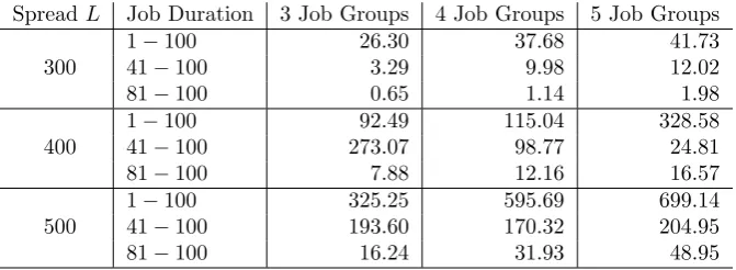
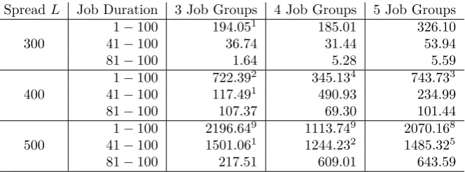
that cannot be solved within one hour will be marked as unsolved. We list only the results on the B&P algorithm because CPLEX cannot solve any of these instances within an hour based on the standard ILP formulation (1)– (5). For each scenario, we show the average computation time (in seconds) of the B&P algorithm. The numbers in superscript represent the number of instances that are not solved within an hour. These results are shown in Tables 1–3. We also show in Table 4 (with the numbers before and after the slashes) the average relative gap at the root node and that after one hour time limit for the case of 3 job groups.
Table 1: Running Time (sec) withn= 100
SpreadL Job Duration 3 Job Groups 4 Job Groups 5 Job Groups
300
1−100 2.31 4.09 2.41
41−100 0.43 0.68 0.44
81−100 0.16 0.16 0.29
400
1−100 14.29 7.72 10.84
41−100 2.41 2.06 4.32
81−100 0.66 0.95 2.17
500
1−100 37.12 20.13 23.63
41−100 13.70 6.52 12.07
[image:14.595.138.474.497.620.2]81−100 1.86 4.23 5.63
Table 2: Running Time (sec) withn= 200
SpreadL Job Duration 3 Job Groups 4 Job Groups 5 Job Groups
300
1−100 26.30 37.68 41.73
41−100 3.29 9.98 12.02
81−100 0.65 1.14 1.98
400
1−100 92.49 115.04 328.58
41−100 273.07 98.77 24.81
81−100 7.88 12.16 16.57
500
1−100 325.25 595.69 699.14
41−100 193.60 170.32 204.95
81−100 16.24 31.93 48.95
in-Table 3: Running Time (sec) withn= 300
SpreadL Job Duration 3 Job Groups 4 Job Groups 5 Job Groups
300
1−100 194.051 185.01 326.10
41−100 36.74 31.44 53.94
81−100 1.64 5.28 5.59
400
1−100 722.392 345.134 743.733 41−100 117.491 490.93 234.99
81−100 107.37 69.30 101.44
500
1−100 2196.649 1113.749 2070.168
41−100 1501.061 1244.232 1485.325
[image:15.595.141.473.158.281.2]81−100 217.51 609.01 643.59
Table 4: Average Relative Gap (%) with 3 Job Groups
SpreadL Job Duration n= 100 n= 200 n= 300
300
1−100 14.25 / 0.00 16.02 / 0.00 12.69 / 1.50 41−100 8.48 / 0.00 11.39 / 0.00 10.67 / 0.00 81−100 6.02 / 0.00 9.36 / 0.00 10.74 / 0.00
400
1−100 14.74 / 0.00 14.65 / 0.00 11.06 / 5.15 41−100 10.29 / 0.00 11.56 / 0.00 6.94 / 1.08 81−100 11.75 / 0.00 10.43 / 0.00 12.42 / 0.00
500
1−100 17.34 / 0.00 14.83 / 0.00 12.01 / 10.43 41−100 13.14 / 0.00 10.52 / 0.00 10.66 / 4.11 81−100 10.88 / 0.00 8.72 / 0.00 9.37 / 0.00
stances with 300 jobs are sometimes difficult, especially in the case with large spread time. In the appendix, we provide a neighborhood search heuristic to be embedded into our B&P algorithm and show that the embedded B&P algorithm runs faster in many difficult scenarios. This heuristic can generate local optimal integer solutions by solving a reduced mixed integer program after randomly removing a number of columns. These local optimal integer solutions help improve the lower bounds and hence speed up the embedded B&P algorithm.
[image:15.595.143.464.337.462.2]Table 5: Total Flexibility with Weights (1, . . . ,1)
Spread Job Machine Distributions Avg#
L Duration in Percentage
300
1−100 15.7 11.0 3.3 7.9 24.3 19.1 10.8 7.2 0.6 0.0 16.4 41−100 30.0 8.5 2.9 7.1 28.4 15.8 4.6 2.1 0.6 0.0 19.7 81−100 31.0 37.4 2.7 4.9 17.0 5.7 0.9 0.5 0.0 0.0 23.0
400
1−100 9.9 8.0 2.4 2.3 22.4 19.7 20.8 10.1 4.5 0.0 13.6 41−100 16.2 11.0 2.1 9.6 24.7 21.6 9.7 3.8 0.7 0.6 16.3 81−100 21.1 9.2 1.6 9.4 31.7 14.9 6.5 5.4 0.0 0.0 18.4
500
1−100 12.1 3.2 1.0 3.3 14.8 20.8 19.9 10.4 11.2 3.3 11.8 41−100 16.6 4.5 1.3 7.9 19.1 23.0 15.9 8.2 3.7 0.0 14.2 81−100 18.1 5.7 0.6 9.8 21.9 26.4 9.5 6.8 1.3 0.0 15.8
4.2. On machine flexibility
Flexibility is one of the most important aspects of production systems. Jordan and Graves [22] study the process flexibility resulted from being able to build different types of products at the same time in the same manufac-turing plant or on the same production line. They show that limited process flexibility may still yield most of the benefits of total process flexibility. In this experiment, we test this statement on machine flexibility for process-ing fixed interval jobs, where the flexibility of a machine is measured by its capability of processing jobs of different classes.
We use the same parameter settings as in the experiment of Section 4.1, except that the number of job groups is set to 10 and the number of jobs is set to 50. The total number of machine classes is c= 210−1 with 10tiers of classes, where each of C10
i = 10!/(i!(10−i)!) tier-i classes consists of those
machines that are each capable of processing jobs ofi job groups. Denote by ˜
Mi the set of machines of tier-iclasses (i= 1, . . . ,10). Therefore, the higher the value of i, the more capable the machines of ˜Mi.
Firstly, using the average number of used machines (Avg#) as an indi-cator, we compare two extreme cases. In one case, we set weights (costs) wi = 1 for all 10 machine sets ˜Mi (i = 1, . . . ,10), while in the other case,
we set the weights to 1 for ˜M1 and the weights to 999 for sets ˜Mi (i ≥ 2).
percentage distribution of used machines across the 10 machine sets.
Table 6: No Flexibility with Weights (1,999, . . . ,999)
Spread Job Machine Distributions Avg#
L Duration in Percentage
300
1−100 100.0 0.0 0.0 0.0 0.0 0.0 0.0 0.0 0.0 0.0 31.7 41−100 100.0 0.0 0.0 0.0 0.0 0.0 0.0 0.0 0.0 0.0 34.0 81−100 100.0 0.0 0.0 0.0 0.0 0.0 0.0 0.0 0.0 0.0 36.5
400
1−100 100.0 0.0 0.0 0.0 0.0 0.0 0.0 0.0 0.0 0.0 27.8 41−100 100.0 0.0 0.0 0.0 0.0 0.0 0.0 0.0 0.0 0.0 30.4 81−100 100.0 0.0 0.0 0.0 0.0 0.0 0.0 0.0 0.0 0.0 31.4
500
1−100 100.0 0.0 0.0 0.0 0.0 0.0 0.0 0.0 0.0 0.0 24.1 41−100 100.0 0.0 0.0 0.0 0.0 0.0 0.0 0.0 0.0 0.0 27.2 81−100 100.0 0.0 0.0 0.0 0.0 0.0 0.0 0.0 0.0 0.0 29.5
We see from Tables 5 and 6 that, when compared with the case of no flexibility, the Avg# values in the case of total flexibility are significantly lower. When there is total flexibility, the selected machines can be freely from all 10 machine sets. In contrast, the selected machines are all from set
˜
M1 (100%) if there is no flexibility.
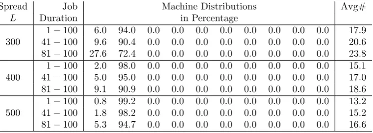
Now let us look at the relationship between machine flexibility and Avg# values. By changing the weights of the machine sets, we gradually increase machine flexibility. The experiment results are shown in Tables 7 and 8.
Table 7: Little Flexibility with Weights (1,1,999, . . . ,999)
Spread Job Machine Distributions Avg#
L Duration in Percentage
300
1−100 6.0 94.0 0.0 0.0 0.0 0.0 0.0 0.0 0.0 0.0 17.9 41−100 9.6 90.4 0.0 0.0 0.0 0.0 0.0 0.0 0.0 0.0 20.6 81−100 27.6 72.4 0.0 0.0 0.0 0.0 0.0 0.0 0.0 0.0 23.8
400
1−100 2.0 98.0 0.0 0.0 0.0 0.0 0.0 0.0 0.0 0.0 15.1 41−100 5.0 95.0 0.0 0.0 0.0 0.0 0.0 0.0 0.0 0.0 17.0 81−100 9.1 90.9 0.0 0.0 0.0 0.0 0.0 0.0 0.0 0.0 18.6
500
[image:17.595.119.500.510.646.2]Table 8: Small Flexibility with Weights (1,1,1,999, . . . ,999)
Spread Job Machine Distributions Avg#
L Duration in Percentage
300
1−100 12.8 7.8 79.4 0.0 0.0 0.0 0.0 0.0 0.0 0.0 16.5 41−100 24.3 23.6 52.0 0.0 0.0 0.0 0.0 0.0 0.0 0.0 19.7 81−100 31.3 38.3 30.4 0.0 0.0 0.0 0.0 0.0 0.0 0.0 23.0
400
1−100 4.0 4.8 91.2 0.0 0.0 0.0 0.0 0.0 0.0 0.0 13.6 41−100 14.4 6.0 79.6 0.0 0.0 0.0 0.0 0.0 0.0 0.0 16.3 81−100 16.4 11.5 72.2 0.0 0.0 0.0 0.0 0.0 0.0 0.0 18.4
500
1−100 4.7 0.8 94.4 0.0 0.0 0.0 0.0 0.0 0.0 0.0 11.8 41−100 11.7 5.4 83.0 0.0 0.0 0.0 0.0 0.0 0.0 0.0 14.2 81−100 11.2 13.8 75.0 0.0 0.0 0.0 0.0 0.0 0.0 0.0 15.8
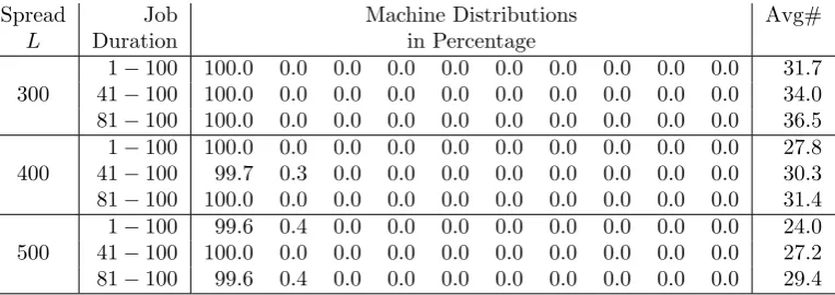
From Tables 7 and 8, we find that limited flexibility can achieve almost the same benefits of total flexibility. As shown in Table 7, the Avg# values are close to the values in Table 5 and those in Table 8 are almost the same as the values in Table 5. Our calculations show that, when machine choices are limited to sets ˜M1 and ˜M2, there is a 92.3% reduction in average Avg# values and, when machine choices are limited to ˜M1, ˜M2 and ˜M3, the reduction
achieves 99.9%! Therefore, higher machine flexibility is almost useless in reducing Avg# values.
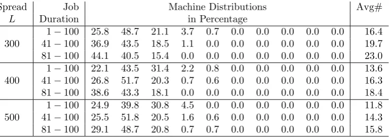
Finally, we examine the impact of more general weights on machine se-lection. We apply a percentage weight increment p when a machine is made capable of processing one more group of jobs. We set the weights to 1 for machines that can process jobs from one group only and the weights to 1+kp for machines which can process k more groups of jobs. Let p = 0.03, 0.20, 0.80 and 1.00, respectively. We present our test results in Tables 9–12.
Table 9: Machine Selection with Weights 1 +kp(k= 0,1, . . . ,9) and p= 0.03
Spread Job Machine Distributions Avg#
L Duration in Percentage
300
1−100 25.6 47.5 23.7 3.1 0.0 0.0 0.0 0.0 0.0 0.0 16.4 41−100 39.3 38.7 21.1 0.9 0.0 0.0 0.0 0.0 0.0 0.0 19.7 81−100 42.8 42.2 15.0 0.0 0.0 0.0 0.0 0.0 0.0 0.0 23.0
400
1−100 21.4 44.3 31.2 3.1 0.0 0.0 0.0 0.0 0.0 0.0 13.6 41−100 30.4 44.0 24.4 1.3 0.0 0.0 0.0 0.0 0.0 0.0 16.3 81−100 37.0 47.0 15.5 0.5 0.0 0.0 0.0 0.0 0.0 0.0 18.4
500
[image:19.595.120.504.374.510.2]1−100 22.4 44.0 30.9 2.7 0.0 0.0 0.0 0.0 0.0 0.0 11.8 41−100 27.6 45.0 25.4 1.9 0.0 0.0 0.0 0.0 0.0 0.0 14.2 81−100 27.7 50.7 19.6 2.1 0.0 0.0 0.0 0.0 0.0 0.0 15.8
Table 10: Machine Selection with Weights 1 +kp(k= 0,1, . . . ,9) andp= 0.20
Spread Job Machine Distributions Avg#
L Duration in Percentage
300
1−100 25.8 48.7 21.1 3.7 0.7 0.0 0.0 0.0 0.0 0.0 16.4 41−100 36.9 43.5 18.5 1.1 0.0 0.0 0.0 0.0 0.0 0.0 19.7 81−100 44.1 40.5 15.4 0.0 0.0 0.0 0.0 0.0 0.0 0.0 23.0
400
1−100 22.1 43.5 31.4 2.2 0.8 0.0 0.0 0.0 0.0 0.0 13.6 41−100 26.8 51.7 20.3 0.7 0.6 0.0 0.0 0.0 0.0 0.0 16.3 81−100 38.6 43.3 18.1 0.0 0.0 0.0 0.0 0.0 0.0 0.0 18.4
500
1−100 24.9 39.8 30.8 4.5 0.0 0.0 0.0 0.0 0.0 0.0 11.8 41−100 25.5 51.8 20.5 1.6 0.6 0.0 0.0 0.0 0.0 0.0 14.3 81−100 29.1 48.7 20.8 0.7 0.7 0.0 0.0 0.0 0.0 0.0 15.8
5. Conclusions
Table 11: Machine Selection with Weights 1 +kp(k= 0,1, . . . ,9) andp= 0.80
Spread Job Machine Distributions Avg#
L Duration in Percentage
300
1−100 36.8 45.6 16.3 0.6 0.7 0.0 0.0 0.0 0.0 0.0 17.5 41−100 53.3 34.4 10.8 1.5 0.0 0.0 0.0 0.0 0.0 0.0 21.3 81−100 63.2 27.0 9.8 0.0 0.0 0.0 0.0 0.0 0.0 0.0 25.0
400
1−100 36.7 40.1 21.9 0.7 0.6 0.0 0.0 0.0 0.0 0.0 14.9 41−100 40.8 43.5 15.1 0.6 0.0 0.0 0.0 0.0 0.0 0.0 17.4 81−100 51.6 38.7 8.7 1.0 0.0 0.0 0.0 0.0 0.0 0.0 19.8
500
[image:20.595.117.499.362.497.2]1−100 31.0 49.9 16.6 2.5 0.0 0.0 0.0 0.0 0.0 0.0 12.7 41−100 40.9 43.2 14.9 1.1 0.0 0.0 0.0 0.0 0.0 0.0 15.5 81−100 37.7 46.9 14.2 1.2 0.0 0.0 0.0 0.0 0.0 0.0 16.6
Table 12: Machine Selection with Weights 1 +kp(k= 0,1, . . . ,9) andp= 1.00
Spread Job Machine Distributions Avg#
L Duration in Percentage
300
1−100 100.0 0.0 0.0 0.0 0.0 0.0 0.0 0.0 0.0 0.0 31.7 41−100 100.0 0.0 0.0 0.0 0.0 0.0 0.0 0.0 0.0 0.0 34.0 81−100 100.0 0.0 0.0 0.0 0.0 0.0 0.0 0.0 0.0 0.0 36.5
400
1−100 100.0 0.0 0.0 0.0 0.0 0.0 0.0 0.0 0.0 0.0 27.8 41−100 99.7 0.3 0.0 0.0 0.0 0.0 0.0 0.0 0.0 0.0 30.3 81−100 100.0 0.0 0.0 0.0 0.0 0.0 0.0 0.0 0.0 0.0 31.4
500
1−100 99.6 0.4 0.0 0.0 0.0 0.0 0.0 0.0 0.0 0.0 24.0 41−100 100.0 0.0 0.0 0.0 0.0 0.0 0.0 0.0 0.0 0.0 27.2 81−100 99.6 0.4 0.0 0.0 0.0 0.0 0.0 0.0 0.0 0.0 29.4
Acknowledgements
Xiandong Zhang thanks the support of National Natural Science Foundation of China (Projects No. 71171058, No. 70832002 and No. 70971100).
References
[1] G. Dantzig, D. Fulkerson, Minimizing the number of tankers to meet a fixed schedule, Naval Research Logistics Quarterly 1 (1954) 217–222.
[2] U. Gupta, D. Lee, J. Leung, An optimal solution for the channel-assignment problem, IEEE Transactions on Computers 100 (1979) 807– 810.
[3] L. Kroon, M. Salomon, L. Van Wassenhove, Exact and approximation algorithms for the operational fixed interval scheduling problem, Euro-pean Journal of Operational Research 82 (1995) 190–205.
[4] L. Kroon, Job Scheduling and Capacity Planning in Aircraft Mainte-nance, PhD Thesis, Rotterdam School of Management, Erasmus Uni-versity, The Netherlands, 1990.
[5] D. Eliiyi, M. Azizoglu, Spread time considerations in operational fixed job scheduling, International Journal of Production Research 44 (2006) 4343–4365.
[6] O. Bekki, M. Azizoglu, Operational fixed interval scheduling problem on uniform parallel machines, International Journal of Production Eco-nomics 112 (2008) 756–768.
[7] D. Eliiyi, M. Azizoglu, A fixed job scheduling problem with machine-dependent job weights, International Journal of Production Research 47 (2009) 2231–2256.
[8] O. Solyali, O. Ozpeynirci, Operational fixed job scheduling problem un-der spread time constraints: a branch-and-price algorithm, International Journal of Production Research 47 (2009) 1877–1893.
[10] L. Kroon, M. Salomon, L. Van Wassenhove, Exact and approximation algorithms for the tactical fixed interval scheduling problem, Operations Research 45 (1997) 624–638.
[11] A. Kolen, L. Kroon, License class design: complexity and algorithms, European Journal of Operational Research 63 (1992) 432–444.
[12] M. Kovalyov, C. Ng, T. Cheng, Fixed interval scheduling: Models, ap-plications, computational complexity and algorithms, European Journal of Operational Research 178 (2007) 331–342.
[13] A. Kolen, J. Lenstra, C. Papadimitriou, F. Spieksma, Interval schedul-ing: A survey, Naval Research Logistics (NRL) 54 (2007) 530–543.
[14] S. Martello, P. Toth, A heuristic approach to the bus driver scheduling problem, European Journal of Operational Research 24 (1986) 106–117.
[15] M. Fischetti, S. Martello, P. Toth, The fixed job schedule problem with spread-time constraints, Operations Research 35 (1987) 849–858.
[16] M. Fischetti, S. Martello, P. Toth, Approximation algorithms for fixed job schedule problems, Operations Research 40 (1992) 96–108.
[17] C. Barnhart, E. L. Johnson, G. L. Nemhauser, M. W. Savelsbergh, P. H. Vance, Branch-and-price: Column generation for solving huge integer programs, Operations Research 46 (1998) 316–329.
[18] E. L. Senne, L. A. Lorena, M. A. Pereira, A branch-and-price approach to p-median location problems, Computers & Operations Research 32 (2005) 1655–1664.
[19] N. Rafiee Parsa, B. Karimi, A. Husseinzadeh Kashan, A branch and price algorithm to minimize makespan on a single batch processing ma-chine with non-identical job sizes, Computers & Operations Research 37 (2010) 1720–1730.
[21] J. Beli¨en, E. Demeulemeester, Scheduling trainees at a hospital depart-ment using a branch-and-price approach, European Journal of Opera-tional Research 175 (2006) 258–278.
[22] W. Jordan, S. Graves, Principles on the benefits of manufacturing pro-cess flexibility, Management Science 41 (1995) 577–594.
[23] A. Caprara, M. Fischetti, P. Toth, A heuristic method for the set cov-ering problem, Operations Research 47 (1999) 730–743.
[24] A. Caprara, P. Toth, M. Fischetti, Algorithms for the set covering problem, Annals of Operations Research 98 (2000) 353–371.
[25] G. Lan, G. DePuy, G. Whitehouse, An effective and simple heuristic for the set covering problem, European Journal of Operational Research 176 (2007) 1387–1403.
Appendix A. An embedding neighborhood search heuristic
In this part, we present a neighborhood search heuristic, abbreviated as NS, that can be embedded into the B&P algorithm for an improved upper bound. The main idea of the NS heuristic is to find randomly some local optimal integer solutions. The best feasible solution is then saved as the current upper bound in the B&P algorithm.
In the column generation step of the B&P algorithm, columns are gener-ated and added to the constraint matrix of the LP relaxation under consid-eration. The NS heuristic generates a local optimal integer solution through a two-step procedure based on the current columns. The idea is similar to those for the set covering problem studied in Caprara et al. [23], Caprara et al. [24] and Lan et al. [25].
Once a better solution is found, the NS will be executed to find the next better solution, if any, in the neighborhood of the best solution so far. This is done iteratively until the number of iterations reaches a given number. After each iteration, if a better ILP solution is identified, all redundant columns, those corresponding to positive components ofXremoval of which still keeps X feasible, will be removed with the largest cost removed first.
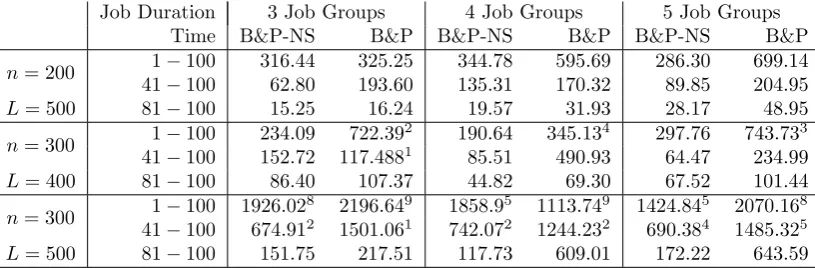
[image:24.595.114.522.358.492.2]Here we used the same problems as in Section 4.1 to test the effectiveness of our embedded B&P algorithm, which we denote by B&P-NS. In this ex-periment, we set θ at 0.6 and the number of iterations at 40 by experience. We present our test results in Table A.13, from which we see that B&P-NS outperforms B&P for all difficult instances and the total number of unsolved instances is reduced by 41%.
Table A.13: Comparison on Running Time (sec)
Job Duration 3 Job Groups 4 Job Groups 5 Job Groups Time B&P-NS B&P B&P-NS B&P B&P-NS B&P
n= 200 1−100 316.44 325.25 344.78 595.69 286.30 699.14 41−100 62.80 193.60 135.31 170.32 89.85 204.95 L= 500 81−100 15.25 16.24 19.57 31.93 28.17 48.95 n= 300 1−100 234.09 722.39
2 190.64 345.134 297.76 743.733
41−100 152.72 117.4881 85.51 490.93 64.47 234.99
L= 400 81−100 86.40 107.37 44.82 69.30 67.52 101.44 n= 300 1−100 1926.02
8 2196.649 1858.95 1113.749 1424.845 2070.168