Linear stationary iterative methods for the force based quasicontinuum approximation

http://wrap.warwick.ac.uk/

Original citation:

Luskin, Mitchell and Ortner, Christoph (2011) Linear stationary iterative methods for the force-based quasicontinuum approximation. In: Engquist, Björn and Runborg, Olof and Tsai, Yen-Hsi R., (eds.) Numerical Analysis of Multiscale Computations. Lecture notes in computational science and engineering, Volume 82 . Berlin : Heidelberg: Springer, pp. 331-368. ISBN 9783642219429.

Permanent WRAP url:

http://wrap.warwick.ac.uk/43774

Copyright and reuse:

The Warwick Research Archive Portal (WRAP) makes this work of researchers of the University of Warwick available open access under the following conditions. Copyright © and all moral rights to the version of the paper presented here belong to the individual author(s) and/or other copyright owners. To the extent reasonable and practicable the material made available in WRAP has been checked for eligibility before being made available.

Copies of full items can be used for personal research or study, educational, or not-for-profit purposes without prior permission or charge. Provided that the authors, title and full bibliographic details are credited, a hyperlink and/or URL is given for the original metadata page and the content is not changed in any way.

Publisher’s statement:

The final publication is available at Springer via http://dx.doi.org/10.1007/978-3-642-21943-6_14

A note on versions:

The version presented here may differ from the published version or, version of record, if you wish to cite this item you are advised to consult the publisher’s version. Please see the ‘permanent WRAP url’ above for details on accessing the published version and note that access may require a subscription.

arXiv:1104.1774v1 [math.NA] 10 Apr 2011

FORCE-BASED QUASICONTINUUM APPROXIMATION

M. LUSKIN AND C. ORTNER

Abstract. Force-based multiphysics coupling methods have become popular since they provide a simple and efficient coupling mechanism, avoiding the difficulties in formulating and implementing a consistent coupling energy. They are also the only known pointwise consistent methods for coupling a general atomistic model to a finite element continuum model. However, the development of efficient and reliable iterative solution methods for the force-based approximation presents a challenge due to the non-symmetric and indefinite structure of the linearized force-based quasicontinuum approximation, as well as to its unusual stability properties. In this paper, we present rigorous numerical analysis and computational experiments to systematically study the stability and convergence rate for a variety of linear stationary iterative methods.

1. Introduction

Low energy local minima of crystalline atomistic systems are characterized by highly localized defects such as vacancies, interstitials, dislocations, cracks, and grain bound-aries separated by large regions where the atoms are slightly deformed from a lattice structure. The goal of atomistic-to-continuum coupling methods [1–4, 15, 16, 22, 26, 28, 32] is to approximate a fully atomistic model by maintaining the accuracy of the atom-istic model in small neighbors surrounding the localized defects and using the efficiency of continuum coarse-grained models in the vast regions that are only mildly deformed from a lattice structure.

Force-based atomistic-to-continuum methods decompose a computational reference lattice into an atomistic region _A and a continuum region_C, and assign forces to rep-resentative atoms according to the region they are located in. In the quasicontinuum method, the representative atoms are all atoms in the atomistic region and the nodes of a finite element approximation in the continuum region. The force-based approxi-mation is thus given by [5, 6, 10–12, 32]

Fjqcf(y) :=

( Fa

j(y) if j ∈ A,

Fc

j(y) if j ∈ C,

Date: April 12, 2011.

2000Mathematics Subject Classification. 65Z05,70C20.

Key words and phrases. atomistic-to-continuum coupling, quasicontinuum method, iterative meth-ods, stability.

This work was supported in part by the National Science Foundation under 0757355, DMS-0811039, the PIRE Grant OISE-0967140, the Institute for Mathematics and Its Applications, and the University of Minnesota Supercomputing Institute. This work was also supported by the De-partment of Energy under Award Number DE-SC0002085. CO was supported by the EPSRC grant EP/H003096/1 “Analysis of Atomistic-to-Continuum Coupling Methods.”

whereydenotes the positions of the representative atoms which are indexed byj,_Fa j(y)

denotes the atomistic force at representative atom j, and _Fc

j(y) denotes a continuum

force at representative atom j.

The force-based quasicontinuum method (QCF) uses a Cauchy-Born strain energy density for the continuum model to achieve a patch test consistent approximation [6, 11, 24]. We recall that a patch test consistent atomistic-to-continuum approximation exactly reproduces the zero net forces of uniformly strained lattices [19, 24, 27]. How-ever, the recently discovered unusual stability properties of the linearized force-based quasicontinuum (QCF) approximation, especially its indefiniteness, present a chal-lenge to the development of efficient and reliable iterative methods [12]. Energy-based quasicontinuum approximations have many attractive features such as more reliable solution methods, but practical patch test consistent, energy-based quasicontinuum approximations have yet to be developed for most problems of physical interest, such as three-dimensional problems with many-body interaction potentials [20, 21, 30].

Rather than attempt an analysis of linear stationary methods for the full nonlinear system, in this paper we restrict our focus to the linearization of a one-dimensional model problem about the uniform deformationyF _{and consider linear stationary}

meth-ods of the form

P u(n+1)₋u(n)=αr(n), (1)

where P is a nonsingular preconditioning operator, the damping parameter α > 0 is fixed throughout the iteration (that is, stationary), and the residual is defined as

r(n) :=f ₋Lqcf_F u(n).

We will see below that our analysis of this simple model problem already allows us to observe many interesting and crucial features of the various methods. For example, we can distinguish which iterative methods converge up to the critical strain F∗ (see (8)

for a discussion of the critical strain), and we obtain first results on their convergence rates.

We begin in Sections 2 and 3 by introducing the most important quasicontinuum ap-proximations and outlining their stability properties, which are mostly straightforward generalizations of results from [9–11, 13]. In Section 4, we review the basic properties of linear stationary iterative methods.

In Section 5, we give an analysis of the Richardson Iteration (P = I) and prove a contraction rate of order 1₋O(N−2_{) in the ℓ}p

ε norm (discrete Sobolev norms are

defined in Section 2.1), where N is the size of the atomistic system.

In Section 6, we consider the iterative solution with preconditioner P =Lqcl_F , where

Lqcl_F is a standard second order elliptic operator, and show that the preconditioned iteration with an appropriately chosen damping parameterα is a contraction up to the critical strain F∗ only in U2,∞ among the common discrete Sobolev spaces. We show,

however, that a rate of contraction in_U2,∞ _{independent ofN can be achieved with the}

elliptic preconditioner Lqcl_F and an appropriate choice of the damping parameter α.

reproduce the stability of the atomistic system [9]. We did not find that the GFC method predicted an instability at a reduced strain in our benchmark tests [18] (see also [24]). To explain this, we note that our 1D analysis in this paper can be considered a good model for cleavage fracture, but not for the slip instabilities studied in [18, 24]. We are currently attempting to develop a 2D benchmark test for cleavage fracture to study the stability of the GFC method.

2. The QC Approximations and Their Stability

We give a review of the prototype QC approximations and their stability properties in this section. The reader can find more details in [9, 10].

2.1. Function Spaces and Norms. We consider a one-dimensional atomistic chain whose 2N+1 atoms have the reference positionsxj =jεforε= 1/N.The displacement

of the boundary atoms will be constrained, so the space of admissible displacements will be given by the displacement space

U =u_∈R2N+1 _{:u−N =uN = 0 .}

We will use various norms on the space _U which are discrete variants of the usual Sobolev norms that arise naturally in the analysis of elliptic PDEs.

For displacements v _{∈ U} and 1_≤p_{≤ ∞}, we define theℓp

ε norms,

kv_kℓp ε :=

  

εPN_ℓ=−N+1|vℓ|p

1/p

, 1_≤p <_∞,

maxℓ=−N+1,...,N|vℓ|, p=∞,

and we denote by _U0,p _{the space U equipped with the ℓ}p

ε norm. The inner product

associated with the ℓ2

ε norm is

hv, w_i:=ε

N

X

ℓ=−N+1

vℓwℓ for v, w∈ U.

We will also use _kf_kℓpε and hf, gito denote the ℓ

p

ε-norm and ℓ2ε-inner product for

arbi-trary vectors f, g which need not belong to _U. In particular, we further define the_U1,p

norm

kv_kU1,p :=kv′k_ℓp ε,

where (v′₎

ℓ =vℓ′ =ε−1(vℓ−vℓ−1),ℓ=−N+ 1, . . . , N, and we letU1,p denote the space

U equipped with the _U1,p _{norm. Similarly, we define the space U}2,p _{and its associated}

U2,p _{norm, based on the centered second difference v}′′

ℓ = ε−2(vℓ+1 −2vℓ +vℓ−1) for

ℓ =₋N + 1, . . . , N ₋1.

We have that v′ _{∈ R}2N _{for v ∈ U has mean zero} PN

j=−N+1vj′ = 0. We can thus

obtain from [10, Equation 9] that

max

v∈U kv′

k_ℓq ε=1

hu′, v′_{i ≤} max

σ∈R2N

kσk_ℓq ε=1

hu′, σ_i=_ku_kU1,p ≤2 max

v∈U kv′

k_ℓq ε=1

We denote the space of linear functionals on _U by _U∗_{. For g ∈ U}∗_{, s = 0,1, and}

1_≤p_{≤ ∞}, we define the negative norms_kg_kU−s,p by

kg_kU−s,p := sup

v∈U kvkUs,q=1

hg, v_i,

where 1_≤q_{≤ ∞} satisfies 1 p +

1

q = 1. We letU

−s,p _{denote the dual space U}∗ _equipped

with the _U−s,p _norm.

For a linear mapping A : _U1 → U2 where Ui are vector spaces equipped with the

norms _{k · k}Ui, we denote the operator norm ofA by

kA_kL(U1,U2) := sup

v∈U, v6=0

kAv_kU2

kv_kU1

.

If _U1 =U2, then we use the more concise notation

kA_kU1 :=kAkL(U1, U1).

If A:_U0,2 _{→ U}0,2 _{is invertible, then we can define the condition numberby}

cond(A) =_kA_kU0,2 · kA−1k_U0,2.

When Ais symmetric and positive definite, we have that cond(A) =λA_2N−1/λA₁

where the eigenvalues of A are 0 < λA

1 ≤ · · · ≤λA2N−1. If a linear mapping A:U → U

is symmetric and positive definite, then we define theA-inner product and A-norm by hv, w_iA:=hAv, wi, kvk2A=hAv, vi.

The operator A : _U1 → U2 is operator stable if the operator norm kA−1kL(U2, U1) is

finite, and a sequence of operators Aj : U1,j → U2,j is operator stable if the sequence

k(Aj)−1kL(U2,j,U1,j) is uniformly bounded. A symmetric operator A : U

0,2 _{→ U}0,2 _is

called stable if it is positive definite, and this implies operator stability. A sequence of positive definite, symmetric operatorsAj :U0,2 → U0,2 is called stable if their smallest

eigenvalues λAj

1 are uniformly bounded away from zero.

2.2. The atomistic model. We now consider a one-dimensional atomistic chain whose 2N+ 3 atoms have the reference positions xj =jε forε= 1/N,and interact only with

their nearest and next-nearest neighbors.

We denote the deformed positions by yj, j =−N −1, . . . , N + 1; and we constrain

the boundary atoms and their next-nearest neighbors to match the uniformly deformed state, yF

j =F jε, whereF > 0 is a macroscopic strain, that is,

y−N−1 =−F(N + 1)ε, y−N =−F Nε,

yN =F Nε, yN+1 =F(N + 1)ε.

(3)

We introduced the two additional atoms with indices _±(N + 1) so that y = yF _{is an}

equilibrium of the atomistic model. The total energy of a deformation y _∈ R2N+3 _is now given by

Ea(y)₋

N

X

j=−N

where

Ea(y)

N_X+1

j=−N

εφyj −yj−1 ε

=

N+1_X

j=−N

εφ(y_j′) +

N+1_X

j=−N+1

εφ(y′_j+y_j′₋₁). (4)

Here,φis a scaled two-body interatomic potential (for example, the normalized Lennard-Jones potential, φ(r) = r−12_−2r−6_{), andf}

j,j =−N, . . . , N, are external forces. The

equilibrium equations are given by the force balance conditions at the unconstrained atoms,

−Fja(ya) =fj for j =−N + 1, . . . , N −1,

ya

j =F jε for j =−N −1, −N, N, N+ 1,

(5)

where the atomistic force (per lattice spacing ε) is given by

Fja(y) : =−

1

ε

∂_Ea_(y)

∂yj

= 1

ε n

φ′(y′_j+1) +φ′(y′_j+2+y′_j+1)₋φ′(y_j′) +φ′(y_j′ +y_j′₋₁) o.

(6)

We linearize (6) by lettingu_∈R2N+3_{,u±N =u±(N+1) = 0, be a “small” displacement} from the uniformly deformed state yF

j =F jε; that is, we define

uj =yj −yjF for j =−N −1, . . . , N + 1.

We then linearize the atomistic equilibrium equations (5) about the uniformly deformed state yF _{and obtain a linear system for the displacement u}a_,

(La_Fua)j =fj for j =−N + 1, . . . , N −1,

ua_j = 0 for j =₋N ₋1, ₋N, N, N + 1,

where (La

Fv)j is given by

(La_Fv)j :=φ′′F

−vj+1+ 2vj−vj−1

ε2

+φ′′_2F

−vj+2+ 2vj −vj−2

ε2

.

Here and throughout we define

φ′′_F :=φ′′(F) and φ′′_2F :=φ′′(2F),

where φ is the interatomic potential in (4). We will always assume that φ′′

F > 0 and

φ′′

2F < 0, which holds for typical pair potentials such as the Lennard-Jones potential

under physically realistic deformations. The stability properties of La

F can be understood by using a representation derived

in [9],

hLa_Fu, u_i=εAF N

X

ℓ=−N+1

|u′_ℓ|2₋ε3φ′′_2F

N

X

ℓ=−N

|u′′_ℓ|2 =AFku′k2ℓ2

ε −ε

2_φ′′

2Fku′′k2ℓ2

ε, (7)

where AF is thecontinuum elastic modulus

We can obtain the following result from the argument in [9, Prop. 1] and [12].

Proposition 1. If φ′′

2F ≤0, then

min

u∈R2N+3_\{0}

u±N=u±(N+1)=0

hLa Fu, ui

ku′_k2 ℓ2

ε

=AF −ε2νεφ′′2F,

where

νε := min u∈R2N+3_\{0} u±N=u±(N+1)=0

ku′′_k2 ℓ2

ε

ku′_k2 ℓ2

ε .

satisfies 0< νε ≤C for some universal constant C.

2.2.1. The critical strain F∗. The previous result shows that LaF is positive definite,

uniformly as N _{→ ∞}, if and only if AF > 0. For realistic interaction potentials, LaF

is positive definite in a ground state F0 > 0. For simplicity, we assume that F0 = 1,

and we ask how far the system can be “stretched” by applying increasing macroscopic strainsF until it loses its stability. In the limit asN _{→ ∞}, this happens at thecritical strain F∗, which is the smallest number larger than F0, solving the equation

AF∗ =φ

′′_(F

∗) + 4φ′′(2F∗) = 0. (8)

2.3. The local QC approximation (QCL). The local quasicontinuum (QCL) ap-proximation uses the Cauchy-Born apap-proximation to approximate the nonlocal atom-istic model by a local continuum model [5, 23, 26]. For next-nearest neighbor interac-tions, the Cauchy-Born approximation reads

φ ε−1(yℓ+1−yℓ−1)

≈ 12

φ(2y_ℓ′) +φ(2y_ℓ+1′ )],

and results in the QCL energy, for y _∈R2N+3 _{satisfying the boundary conditions (3),}

Eqcl(y) =

N

X

j=−N+1

εφ(y_j′) +φ(2y′_j)

+ε

φ(y₋′ _N) + 1 2φ(2y

′

−N) +φ(yN′ +1) +

1 2φ(2y

′ N+1)

.

(9)

Imposing the artificial boundary conditions of zero displacement from the uniformly deformed state, yF

j =F jε, we obtain the QCL equilibrium equations

−Fjqcl(yqcl) =fj for j =−N + 1, . . . , N −1,

y_jqcl =F jε for j =₋N, N,

where

Fjqcl(y) : =−

1

ε

∂_Eqcl_(y)

∂yj

= 1

ε n

φ′(y′_j+1) + 2φ′(2y_j+1′ )₋φ′(y_j′) + 2φ′(2y′_j) o.

We see from (10) that the QCL equilibrium equations are well-defined with only a single constraint at each boundary, and we can restrict our consideration to

y_∈R2N+1 _{with y−N =−F and yN =F as the boundary conditions.}

Linearizing the QCL equilibrium equations (10) about yF _{results in the system}

(Lqcl_F uqcl)j =fj for j =−N + 1, . . . , N −1,

uqcl_j = 0 for j =₋N, N,

where

Lqcl_F =AFL

and L is the discrete Laplacian, for v _{∈ U}, given by

(Lv)j :=−v′′j =

−vj+1+ 2vj −vj−1

ε2

, j =₋N + 1, . . . , N ₋1. (11)

The QCL operator is a scaled discrete Laplace operator, so

hLqcl_F u, u_i=AFku′k2ℓ2

ε for all u∈ U.

In particular, it follows that Lqcl_F is stable if and only if AF >0, that is, if and only if

F < F∗, where F∗ is the critical strain defined in (8).

2.4. The force-based QC approximation (QCF). The force-based quasicontin-uum (QCF) method combines the accuracy of the atomistic model with the efficiency of the QCL approximation by decomposing the computational reference lattice into an atomistic region_A and acontinuum region _C, and assigns forces to atoms according to the region they are located in. The QCF operator is given by [5, 6]

Fjqcf(y) :=

( Fa

j(y) if j ∈ A,

Fjqcl(y) ifj ∈ C,

(12)

and the QCF equilibrium equations are given by

−Fjqcf(yqcf) = fj for j =−N + 1, . . . , N −1,

y_jqcf =F jε for j =₋N, N.

We note that, since atoms near the boundary belong to_C, only one boundary condition is required at each end.

For simplicity, we specify the atomistic and continuum regions as follows. We fix

K _∈N_{, 1≤K ≤N −2, and define}

A =_{−K, . . . , K_} and _C =_{−N + 1, . . . , N ₋1_{} \ A}.

Linearizing (12) about yF_{, we obtain}

(Lqcf_F uqcf)j =fj for j =−N + 1, . . . , N −1,

uqcf_j = 0 for j =₋N, N, (13)

where the linearized force-based operator is given explicitly by

(Lqcf_F v)j :=

(Lqcl_F v)j, for j ∈ C,

(La

The stability analysis of the QCF operator Lqcf_F is less straightforward [10, 11]; we will therefore treat it separately and postpone it to Section 3.

2.5. The original energy-based QC approximation (QCE). The original energy-based quasicontinuum (QCE) method [26] defines an energy functional by assigning atomistic energy contributions in the atomistic region and continuum energy contribu-tions in the continuum region. For our model problem, we obtain

Eqce(y) =εX

ℓ∈A

Eℓa(y) +ε

X

ℓ∈C

Eℓc(y) for y∈R2N+1,

where

Eℓc(y) = 12 φ(2y ′

ℓ) +φ(yℓ′) +φ(yℓ+1′ ) +φ(2yℓ+1′ )

, and Eℓa(y) = 12 φ(y

′

ℓ−1+yℓ′) +φ(y′ℓ) +φ(y′ℓ+1) +φ(yℓ+1′ +yℓ+2′ )

.

The QCE method is patch tests inconsistent [7,8,25,31], which can be seen from the existence of “ghost forces” at the interface, that is, _∇Eqce_(yF_{) = g}F _{6= 0. Hence, the}

linearization of the QCE equilibrium equations aboutyF _{takes the form (see [8, Section}

2.4] and [7, Section 2.4] for more detail)

(Lqce_F uqce)j −gjF =fj for j =−N + 1, . . . , N −1,

uqce_j = 0 for j =₋N, N, (14)

where, for 0 _≤j _≤N ₋1, we have

(Lqce_F v)j =φ′′F−

vj+1+ 2vj −vj−1

ε2

+φ′′_2F                                 

4−vj+2+ 2vj−vj−2

4ε2 , 0≤j ≤ K−2,

4−vj+2+ 2vj−vj−2 4ε2 +

1

ε

vj+2−vj

2ε , j =K −1,

4−vj+2+ 2vj−vj−2 4ε2 −

2

ε

vj+1−vj

ε +

1

ε

vj+2−vj

2ε , j =K,

4−vj+1+ 2vj−vj−1

ε2 −

2

ε

vj −vj−1

ε +

1

ε

vj−vj−2

2ε , j =K+ 1,

4−vj+1+ 2vj−vj−1

ε2 +

1

ε

vj−vj−2

2ε , j =K+ 2,

4−vj+1+ 2vj−vj−1

ε2 , K+ 3 ≤j ≤N −1,

and where the vector of “ghost forces,” g, is defined by

g_jF =                   

0, 0_≤j _≤K₋2,

−1 2εφ

′

2F, j=K−1, 1

2εφ ′

2F, j=K,

1 2εφ

′

2F, j=K+ 1,

−2ε1φ′2F, j=K+ 2,

0, K+ 3 _≤j _≤N ₋1.

The following result is a new sharp stability estimate for the QCE operator Lqce_F . Its somewhat technical proof is given in Appendix 8.1.

Theorem 2. If K _≥1, N _≥K+ 2, andφ′′

2F ≤0, then

inf

u∈U ku′

k_ℓ2

ε=1

hLqce_F u, u_i=AF +λKφ′′2F,

where 1

2 ≤λK ≤1. Asymptotically, as K → ∞, we have

λK ∼λ∗+O(e−cK) where λ∗ ≈0.6595 and c≈1.5826.

2.6. The quasi-nonlocal QC approximation (QNL). The QCF method is the simplest idea to circumvent the interface inconsistency of the QCE method, but gives non-conservative equilibrium equations [5]. An alternative energy-based approach was suggested in [14, 33], which is based on a modification of the energy at the interface. The quasi-nonlocal approximation (QNL) is given by the energy functional

Eqnl(y) :=ε

N

X

ℓ=−N+1

φ(y′ℓ) +ε

X

ℓ∈A

φ(yℓ′ +yℓ+1′ ) +ε

X

ℓ∈C 1 2

φ(2y′ℓ) +φ(2y′ℓ+1)

,

where we set φ(y′

−N) =φ(yN+1′ ) = 0. The QNL approximation is patch test consistent;

that is, y=yF _{is an equilibrium of the QNL energy functional.}

The linearization of the QNL equilibrium equations about yF _is

(Lqnl_F uqnl₎

j =fj for j =−N + 1, . . . , N −1,

uqnl_j = 0 for j =₋N, N,

where

(Lqnl_F v)j =φ′′F−

vj+1+ 2vj −vj−1

ε2

+φ′′_2F                   

4−vj+2+ 2vj−vj−2

4ε2 , 0≤j ≤K−1,

4−vj+2+ 2vj−vj−2 4ε2 −

−vj+2+ 2vj+1−vj

ε2 , j =K,

4−vj+1+ 2vj−vj−1

ε2 +

−vj + 2vj−1−vj−2

ε2 , j =K+ 1,

4−vj+1+ 2vj−vj−1

ε2 , K+ 2 ≤j ≤N −1.

(15)

We can repeat our stability analysis for the periodic QNL operator in [9, Sec. 3.3] verbatim to obtain the following result.

Proposition 3. If K < N ₋1, and φ2F ≤0, then

inf

u∈U ku′

k_ℓ2

ε=1

Remark 1. _{Since φ}′′

2F = (AF −φ′′F)/4,the linearized operators (φF′′)−1LaF,(φ′′F)−1L qcl F ,

(φ′′ F)−1L

qcf

F ,(φ′′F)−1L qce

F ,and (φ′′F)−1L qnl

F depend only on AF/φ′′F, N and K.

3. Stability and Spectrum of the QCF operator

In this section, we give various properties of the linearized QCF operator, most of which are variants of our results in [10,11]. We first give a result for the non-coercivity of the QCF operator which lies at the heart of many of the difficulties one encounters in analyzing the QCF method.

Theorem 4 (Theorem 1, [11]). If φ′′

F >0 and φ′′2F ∈R\ {0} then, for sufficiently

large N, the operator Lqcf_F is not positive-definite. More precisely, there exist N0 ∈ N

and C1 ≥C2 >0 such that, for all N ≥N0 and 2≤K ≤N/2,

−C1N1/2 ≤ inf v∈U kv′

k_ℓ2

ε=1

Lqcf_F v, v _{≤ −}C2N1/2.

The proof of Theorem 4 yields also the following asymptotic result on the operator norm of Lqcf_F . Its proof is a straightforward extension of [11, Lemma 2], which covers the case p= 2, and we therefore omit it.

Lemma 5. Let φ′′

2F 6= 0, then there exists a constant C3>0 such that for sufficiently

large N, and for 2_≤K _≤N/2,

C₃−1N1/p _≤Lqcf_{F L(U}1,p_,U−1,p₎ ≤C3N

1/p_.

As a consequence of Theorem 4 and Lemma 5, we analyzed the stability of Lqcf_F in alternative norms. By following the proof of [10, Theorem 3] verbatim (see also [10, Remark 3]), we can obtain the following sharp stability result.

Proposition 6. If AF >0 and φ′′2F ≤0, then L qcf

F is invertible with

(Lqcf_F )−1_L(U0,∞_{, U}2,∞₎ ≤1/AF.

If AF = 0, then LqcfF is singular.

This result shows that Lqcf_F is operator stable up to the critical strain F∗ at which

the atomistic model loses its stability as well (cf. Section 2.2).

3.1. Spectral properties of Lqcf_F in _U0,2 _{= ℓ}2

ε. The spectral properties of the L qcf F

operator are fundamental for the analysis of the performance of iterative methods in Hilbert spaces. The basis of our analysis of Lqcf_F in the Hilbert space _U0,2 _{is the}

given in [13, Section 3], which translates verbatim to the case of Dirichlet boundary conditions and yields the following result.

Lemma 7. For all N _≥4, 1_≤K _≤N ₋2, we have the identity

Lqcf_F =L−1Lqnl_F L. (16)

In particular, the operator Lqcf_F is diagonalizable and its spectrum is identical to the spectrum of Lqnl_F .

We denote the eigenvalues of Lqnl_F (and Lqcf_F ) by

0< λqnl1 ≤...λ qnl

ℓ ≤...≤λ qnl 2N−1.

The following lemma gives a lower bound for λqnl₁ , an upper bound for λqnl_2N−1, and consequently an upper bound for cond(Lqnl_F ) =λqnl_2N−1/λqnl₁ .

Lemma 8. If K < N₋1 and φ′′

2F ≤0, then

λqnl_{1 ≥}2AF, λqnl2N−1 ≤(AF −4φ′′2F)ε−2 =φ′′Fε−2, and

cond(Lqnl_F ) = λ

qnl 2N−1

λqnl₁ ≤

φ′′ F

2AF

ε−2.

For the analysis of iterative methods, we are also interested in the condition number of a basis of eigenvectors of Lqcf_F as N tends to infinity. Employing Lemma 7, we can write Lqcf_F = L−1_Λqcf_{L where L is the discrete Laplacian operator and Λ}qcf _is

diagonal. The columns of L−1 _{are poorly scaled; however, a simple rescaling was}

found in [13, Thm. 3.3] for periodic boundary conditions. The construction and proof translate again verbatim to the case of Dirichlet boundary conditions and yield the following result (note, in particular, that the main technical step, [13, Lemma 4.6] can be applied directly).

Lemma 9. LetAF >0, then there exists a matrixV of eigenvectors for the force-based

QC operator Lqcf_F such thatcond(V) is bounded above by a constant that is independent of N.

3.2. Spectral properties of Lqcf_F in _U1,2_{. In our analysis below, particularly in}

Sec-tions 6.1 and 6.2, we will see that the preconditioner Lqcl_F = AFL is a promising

candidate for the efficient solution of the QCF system. The operator L1/2 _{can be}

un-derstood as a basis transformation to an orthonormal basis in _U1,2_{. Hence, it will be}

useful to study the spectral properties ofLqcf_F in that space. The relevant (generalized) eigenvalue problem is

Lqcf_F v =λLv, v _{∈ U}, (17)

which can, equivalently, be written as

L−1Lqcf_F v =λv, v _{∈ U}, (18) or as

L−1/2_Lqcf

with the basis transformw=L1/2_{v, in either case reducing it to a standard eigenvalue}

problem in ℓ2

ε. Since L and L1/2 commute, Lemma 7 immediately yields the following

result.

Lemma 10. For all N _≥4, 1 _≤K _≤ N ₋2 the operator L−1_Lqcf

F is diagonalizable

and its spectrum is identical to the spectrum of L−1_Lqnl F .

We gave a proof in [12] of the following lemma, which completely characterizes the spectrum of L−1_Lqnl

F , and thereby also the spectrum of L−1L qcf

F . We denote the

spectrum of L−1_Lqnl

F (and L−1L qcf

F ) by {µ qnl

j :j = 1, . . . ,2N −1}.

Lemma 11. Let K _≤N ₋2 and AF >0, then the (unordered) spectrum of L−1Lqnl_F

(that is, the _U1,2_{-spectrum) is given by}

µqnl_j = (

AF −4φ′′2F sin2 jπ 4K+4

, j = 1, . . . ,2K+ 1, AF, j = 2K+ 2, . . . ,2N −1.

In particular, if φ′′

2F ≤0, then

maxjµqnlj

minjµqnlj

= 1₋ 4φ

′′ 2F

AF

sin2(2K+1)π_4K+4 = φ

′′ F

AF

+4φ

′′ 2F

AF

sin2 _4K+4π = φ

′′ F

AF

+O(K−2).

We conclude this study by stating a result on the condition number of the matrix of eigenvectors for the eigenvalue problem (19). Letting ˜V be an orthogonal matrix of eigenvectors of L−1/2_Lqnl

F L−1/2 and ˜Λ the corresponding diagonal matrix, then Lemma

7 yields

L−1/2Lqcf_F L−1/2 = L−1L−1/2Lqnl_F L−1/2L

= ( ˜VTL)−1Λ( ˜˜ VTL).

Clearly, cond( ˜VT_{L) =O(N}2_{), which gives the following result.}

Lemma 12. If AF > 0, then there exists a matrix Wf of eigenvectors for the

preconditioned force-based QC operator L−1/2_Lqcf

F L−1/2, such that cond(fW) = O(N2)

as N _{→ ∞}.

4. Linear Stationary Iterative Methods

In this section, we investigate linear stationary iterative methods to solve the lin-earized QCF equations (13). These are iterations of the form

P u(n)₋u(n−1)=αr(n−1), (20) where P is a nonsingular preconditioner, the step size parameter α > 0 is constant (that is, stationary), and the residual is defined as

r(n) :=f ₋Lqcf_F u(n).

The iteration error

satisfies the recursion

P e(n) = P ₋αLqcf_F e(n−1),

or equivalently,

e(n) = I₋αP−1Lqcf_F e(n−1) =:Ge(n−1), (21) where the operator G = I ₋αP−1_Lqcf

F : U → U is called the iteration matrix. By

iterating (21), we obtain that

e(n) = I ₋αP−1Lqcf_F ne(0) =Gne(0). (22) Before we investigate various preconditioners, we briefly review the classical theory of linear stationary iterative methods [29]. We see from (22) that the iterative method (20) converges for every initial guess u(0) _{∈ U if and only if G}n _{→ 0 asn → ∞. For a}

given norm _kv_k, for v _{∈ U}, we can see from (22) that the reduction in the error after

n iterations is bounded above by

kGn_k= sup

e(0)_∈U

ke(n)_k

ke(0)_k.

It can be shown [29] that the convergence of the iteration for every initial guess

u(0) _{∈ U is equivalent to the condition ρ(G) <1, where ρ(G) is the spectral radius of}

G,

ρ(G) = max_{|λi|:λi is an eigenvalue of G}.

In fact, the Spectral Radius Theorem [29] states that

lim

n→∞kG n

k1/n =ρ(G)

for any vector norm on _U. However, if ρ(G) < 1 and _kG_{k ≥} 1, the Spectral Radius Theorem does not give any information about how largenmust be to obtain_kGn_{k ≤1.}

On the other hand, if ρ(G) < 1, then there exists a norm _{k · k} such that _kG_k < 1, so that G itself is a contraction [17]. In this case, we have the stronger contraction property that

ke(n)_{k ≤ k}G_kke(n−1)_{k ≤ k}G_kn_ke(0)_k.

In the remainder of this section, we will analyze the norm of the iteration matrix, kG_k, for several preconditionersP, using appropriate norms in each case.

5. The Richardson Iteration (P =I)

The simplest example of a linear iterative method is the Richardson iteration, where

P =I. If follows from Lemma 9 that there exists a similarity transform S such that

Lqcf_F =S−1ΛqnlS, (23)

where cond(S) _≤ C (where C is independent of N), and Λqnl _{is the diagonal matrix}

of _U0,2_{-eigenvalues (λ}qnl

j )2Nj=1−1 of L qcf

F . As an immediate consequence, we obtain the

identity

Gid(α) = I−αLqcfF =S −1 _I

−αΛqnlS,

where yields

kGid(α)kℓ2

ε ≤cond(S)kI−αΛ

qnl

kℓ2

ε ≤C max

j=1,...,2N−1

If AF > 0, then it follows from Proposition 3 that λqnlj > 0 for all j, and hence that

the iteration matrixGid(α) :=I−αLqcfF is a contraction in the k · kℓ2

ε norm if and only

if 0< α < αid

max:= 2/λ qnl

2N−1. It follows from Lemma 8 thatαidmax≤(2ε2)/φ′′F.

We can minimize the contraction constant forGid(α) in thekvkST_Snorm by choosing α=αidopt := 2/(λ

qnl

1 +λ

qnl

2N−1), and in this case we obtain from Lemma 8 that

Gid αoptid _ℓ2

ε ≤C

λqnl_2N−1−λqnl₁ λqnl_2N−1+λqnl₁ ≤C

1₋ 2AFε

2

φ′′ F

.

It thus follows that the contraction constant forGid(α) in thek · kℓ2

ε norm is only of the

order 1₋O(ε2_{), even with an optimal choice of α. This is the same generic behavior}

that is typically observed for Richardson iterations for discretized second-order elliptic differential operators.

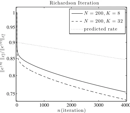
5.1. Numerical example for the Richardson Iteration. In Figure 1, we plot the error in the Richardson iteration against the iteration number. As a typical example, we use the right-hand side

f(x) =h(x) cos(3πx) where h(x) = (

1, x_≥0,

−1, x <0, (25)

which is smooth in the continuum region but has a discontinuity in the atomistic region. We choose φ′′

F = 1, AF = 0.5, and the optimal α = αidopt discussed above (we

note that Gid(αidopt) depends only on AF/φF′′ and N, but e(0) depends on AF and φ′′F

independently) . We observe initially a much faster convergence rate than the one predicted because the initial residual for (25) has a large component in the eigenspaces corresponding to the intermediate eigenvalues λqnl_j for 1 < j <2N ₋1. However, after a few iterations the convergence behavior approximates the predicted rate.

6. Preconditioning with QCL (P =Lqcl_F =AFL)

We have seen in Section 5 that the Richardson iteration with the trivial precondi-tionerP =I converges slowly, and with a contraction rate of the order 1₋O(ε2_{). The}

goal of a (quasi-)optimal preconditioner for large systems is to obtain a performance that is independent of the system size. We will show in the present section that the preconditioner P = AFL (the system matrix for the QCL method) has this desirable

quality.

Of course, preconditioning with P =AFLcomes at the cost of solving a large linear

system at each iteration. However, the QCL operator is a standard elliptic operator for which efficient solution methods exist. For example, the preconditioner P =AFL

could be replaced by a small number of multigrid iterations, which would lead to a solver with optimal complexity. Here, we will ignore these additional complications and assume that P is inverted exactly.

Throughout the present section, the iteration matrix is given by

Gqcl(α) :=I−α(LqclF )−1L qcf

0 1000 2000 3000 4000 0.75

0.8 0.85 0.9 0.95 1

Richardson Iteration

n(iteration)

k

e

(

n

)k

ℓ

2ǫ

/

k

e

(

0

)k

ℓ

2ǫ

N= 200, K= 8

N= 200, K= 32

predicted rate

Figure 1. Normalized ℓ2

ε-error of successive Richardson iterations for

the linear QCF system with N = 200, K = 8, 32, φ′′

F = 1, AF = 0.5,

optimal α=αid

opt,right-hand side (25), and starting guess u(0)= 0.

where α > 0 and AF =φF′′ + 4φ′′2F >0. We will investigate whether, if U is equipped

with a suitable topology, Gqcl(α) becomes a contraction. To demonstrate that this is

a non-trivial question, we first show that in the spaces _U1,p_{, 1 ≤ p < ∞, which are}

natural choices for elliptic operators, this result does not hold.

Proposition 13. If 2_≤K _≤N/2, φ′′

2F 6= 0, and p ∈[1,∞), then for any α > 0 we

have

kGqcl(α)k_U1,p ∼N1/p as N → ∞.

Proof. We have from (2) andq =p/(p₋1) the inequality

L−1Lqcf_{F U}1,p = max

u∈U ku′

k_ℓp ε=1

L−1Lqcf_F u′_ℓp ε

≤ 2 max

u,v∈U ku′

k_ℓp ε=1,kv

′

k_ℓq ε=1

D

L−1Lqcf_F u′, v′E

= 2 max

u,v∈U ku′

k_ℓp ε=1,kv

′

k_ℓq ε=1

D

L L−1Lqcf_F u, vE

= 2 max

u,v∈U ku′

k_ℓp ε=1,kv

′

k_ℓq ε=1

Lqcf_F u, v

= 2Lqcf_{F L(U}1,p_,U−1,p₎

as well as the reverse inequality

Lqcf_{F L(U}1,p_{, U}−1,p₎≤

The result now follows from the definition of Gqcl(α) in (26), Lemma 5, and the fact

that α >0 and AF >0.

We will return to an analysis of the QCL preconditioner in the space _U1,2 _{in Section}

6.3, but will first attempt to prove convergence results in alternative norms.

6.1. Analysis of the QCL preconditioner in _U2,∞_{. We have found in our previous}

analyses of the QCF method [10, 11] that it has superior properties in the function spaces _U1,∞ _{and U}2,∞_{. Hence, we will now investigate whether α can be chosen such}

that Gqcl(α) is a contraction, uniformly as N → ∞. In [10], we have found that

the analysis is easiest with the somewhat unusual choice _U2,∞_{. Hence we begin by}

analyzing Gqcl(α) in this space.

To begin, we formulate a lemma in which we compute the operator norm of Gqcl(α)

explicitly. Its proof is slightly technical and is therefore postponed to Appendix 8.2.

Lemma 14. If N _≥4, then

kGqcl(α)k_U2,∞ =

1₋α 1₋2φ′′2F

AF

_+α2φ′′

2F

AF

.

What is remarkable (though not necessarily surprising) about this result is that the operator norm of Gqcl(α) is independent of N and K. This immediately puts us into

a position where we can obtain contraction properties of the iteration matrix Gqcl(α),

that are uniform inN and K. It is worth noting, though, that the optimal contraction rate is not uniform as AF approaches zero; that is, the preconditioner does not give

uniform efficiency as the system approaches its stability limit.

Theorem 15. Suppose that N _≥4, AF >0, and φ′′2F ≤0, and define

αqcl,2,_opt ∞ := AF

AF + 2|φ′′2F|

= 2AF

φ′′ F +AF

and α_maxqcl,2,∞:= 2AF

φ′′ F

.

Then Gqcl(α) is a contraction of U2,∞ if and only if 0 < α < αqcl,2,max ∞, and for any

such choice the contraction rate is independent of N and K. The optimal choice is

α=αqcl,2,_opt ∞, which gives the contraction rate

Gqcl αqcl,2,opt ∞_U2,∞ =

1−AF_φ′′ F

1+AF

φ′′ F

<1.

Proof. Note that αoptqcl,2,∞ = 1/ 1− 2φ′′

2F

AF

. Hence, if we assume, first, that 0 < α _≤ α_optqcl,2,∞, then

kGqcl(α)kU2,∞ = 1−α 1−2φ ′′

2F

AF

−2αφ′′2F

AF = 1−α=:m1(α).

The optimal choice is clearly α=αqcl,2,_opt ∞ which gives the contraction rate

Gqcl αqcl,2,opt ∞_U2,∞ =α

qcl,2,∞ opt

2φ

′′ 2F

AF

= 2|φ

′′ 2F|

φ′′

F + 2φ′′2F

= 1−

AF φ′′ F

1+AF

Alternatively, if α_≥α_optqcl,2,∞, then

Gqcl(α)

U2,∞ =α 1−

4φ′′

2F

AF

−1 =αφ

′′ F

AF −

1 =:m2(α).

This value is strictly increasing with α, hence the optimal choice is againα=α_optqcl,2,∞. Moreover, we have m2(α)<1 if and only if

α < 2AF φ′′

F

=αqcl,2,_max∞.

Since, for α = αqcl,2,_opt ∞ we have m1(α) = m2(α) <1, it follows that αmaxqcl,2,∞ > α qcl,2,∞ opt

(as a matter of fact, the condition αqcl,2,∞ max > α

qcl,2,∞

opt is equivalent to AF > 0). In

conclusion, we have shown that _kGqcl(α)kU2,∞ is independent ofN and K and that it

is strictly less than one if and only if α < αqcl,2,∞

max , with optimal value α=α qcl,2,∞

opt .

As an immediate corollary, we obtain the following general convergence result.

Corollary 16. Suppose that N _≥ 4, AF > 0, φ′′2F ≤ 0, and suppose that k · kX is a

norm defined on _U such that

ku_kX ≤CkukU2,∞ ∀u∈ U.

Moreover, suppose that 0< α < αqcl,2,∞

max . Then, for any u∈ U,

kGqcl(α)nuk_X ≤qˆnCkukU2,∞ →0 as n → ∞,

where qˆ:=_kGqcl(α)kU2,∞ <1.

In particular, the convergence is uniform among all N, K and all possible initial values u_{∈ U} for which a uniform bound on _ku_kU2,∞ holds.

Proof. We simply note that, according to Theorem 15, for 0< α < αqcl,2,∞

max , we have

kGqcl(α)nk_U2,∞ ≤qˆn,

where ˆq:=_kGqcl(α)kU2,∞ <1 is a number that is independent ofN and K. Hence, we

have

kGqcl(α)nuk_X ≤CkGqcl(α)nuk_U2,∞ ≤Cqˆnkuk_U2,∞.

Remark 2. _{Although we have seen in Theorem 15 and Corollary 16 that the linear}

stationary method with preconditioner AFL and with sufficiently small step size α

is convergent, this convergence may still be quite slow if the initial data is “rough.” Particularly in the context of defects, we may, for example, be interested in the con-vergence properties of this iteration when the initial residual is small or moderate in U1,p_{, for some p ∈ [1,∞], but possibly of order O(N) in the U}2,∞_{-norm. We can see}

from the following Poincar´e and inverse inequalities

ku_kU1,∞ ≤ 1

2kukU2,∞ and kukU2,∞ ≤2NkukU1,∞ for all u∈ U; that the application of Corollary 16 to the case X =_U1,∞ _{gives the estimate}

Similarly, with X =_U1,2_{, we obtain}

kGqcl(α)nuk_U1,2 ≤qˆnN3/2kukU1,2 for all u∈ U. (27)

We have seen in Proposition 13 that a direct convergence analysis in _U1,p_{, p < ∞,}

may be difficult with analytical methods, hence we focus in the next section on the

case _U1,∞_.

6.2. Analysis of the QCL preconditioner in _U1,∞_{. As before, we first compute}

the operator norm of the iteration matrix explicitly. The proof of the following lemma is again postponed to the Appendix 8.2.

Lemma 17. If K _≥3, N _≥max(9, K+ 3), and φ′′

2F ≤0, then

kGqcl(α)k_U1,∞ =   

1₋α+α4φ′′2F

AF

for 0_≤α_≤αqcl,1,_opt ∞,

1₋α 1₋2φ′′2F

AF +α(6 + 2ε−4εK)

φ′′

2F

AF

for αqcl,1,_opt ∞ _≤α,

where

αqcl,1,_opt ∞ :=h1 + (2 +ε₋2εK)φ′′2F

AF

i−1

satisfies αqcl,2,_opt ∞_≤αqcl,1,_opt ∞_≤1.

Again we note that the operator norm is independent, but now up to terms of order O(εK), of the system size.

Theorem 18. Suppose that K _≥ 3, N _≥ max(9, K + 3), and φ′′

2F < 0, then the

following statements are true: (i) If φ′′

F + 8φ′′2F ≤0,then Gqcl(α)isnot a contraction ofU1,∞, for any value ofα.

(ii) If φ′′

F + 8φ′′2F >0, then Gqcl(α) is a contraction for sufficiently small α. More

precisely, setting

αqcl,1,max∞ :=

2AF

AF + (8 + 2ε−4εK)|φ′′2F|

,

we have that Gqcl(α) is a contraction of U1,∞ if and only if 0 < α < αqcl,1,max∞.

The operator norm _kGqcl(α)kU1,∞ is minimized by choosing α = αqcl,1,∞

opt (cf.

Lemma 17) and in this case

Gqcl αqcl,1,opt ∞_U1,∞ = 1−

φ′′

F + 8φ′′2F

φ′′

F + (2−ε+ 2εK)φ′′2F

<1.

Proof. Suppose, first, that 0< α_≤αqcl,1,opt ∞. Since αqcl,1,opt ∞≤1 it follows that

Gqcl(α)

U1,∞ = 1−α φ′′

F + 8φ′′2F

AF

,

and hence _kGqcl(α)kU1,∞ <1 if and only if φ′′

F + 8φ′′2F >0. In that case kGqcl(α)kU1,∞

is strictly decreasing in (0, αqcl,1,opt ∞].

Sinceα_optqcl,1,∞_≥α_optqcl,2,∞= (1₋2φ′′2F

AF)

−1_{we can see thatkG}

qcl(α)kU1,∞ is always strictly

increasing in [αqcl,1,opt ∞,+∞) and hence if φ′′F + 8φ′′2F > 0, then α = α qcl,1,∞

the operator norm _kGqcl(α)kU1,∞. Moreover, straightforward computations show that αqcl,1,∞

max > α qcl,1,∞

opt and that kGqcl(α)kU1,∞ <1 if and only if 0 < α < αqcl,1,∞

max .

We remark that the optimal value of α in _U1,∞_{, that is α = α}qcl,1,∞

opt , is not the

same as the optimal value, αqcl,2,opt ∞, inU2,∞. However, it is easy to see that α qcl,1,∞

opt =

α_optqcl,2,∞+O(εK), and hence, even though αqcl,2,_opt ∞is not optimal in _U1,∞ _{it is still close}

to the optimal value. On the other hand, αqcl,1,∞

max and αqcl,2,max∞ are not close, since, if

4εK ₋2ε <1,then

αqcl,1,_max∞_≤ 2AF φ′′

F + 3|φ′′2F|

< 2AF φ′′

F

=αqcl,2,_max ∞.

In summary, we have seen that the contraction property of Gqcl(α) in U1,∞ is

signif-icantly more complicated than in _U2,∞_{, and that, in fact, G}

qcl(α) is not a contraction

for all macroscopic strains F up to the critical strain F∗.

6.3. Analysis of the QCL preconditioner in _U1,2_{. Even though we were able}

to prove uniform contraction properties for the QCL-preconditioned iterative method in _U2,∞_{, we have argued above that these are not entirely satisfactory in the}

pres-ence of irregular solutions containing defects. Hpres-ence we analyzed the iteration matrix

Gqcl(α) =I−α(AFL)−1LqcfF in U1,∞, but there we showed that it is not a contraction

up to the critical load F∗. To conclude our results for the QCL preconditioner, we

present a discussion of Gqcl(α) in the space U1,2.

We begin by noting that it follows from (21) that

P1/2e(n) = P1/2Gqcl(α)e(n−1) =P1/2

I₋αP−1Lqcf_F P−1/2 P1/2e(n−1)

= I₋αP−1/2L_FqcfP−1/2 P1/2e(n−1)=:Geqcl(α) P1/2e(n−1).

Since _kP1/2_vk ℓ2

ε = A

1/2

F kvkU1,2 for v ∈ U, it follows that G_qcl(α) is a contraction in

U1,2 _{if and only if G}e

qcl(α) is a contraction in ℓ2ε. Unfortunately, we have shown in

Proposition 13 that _kGqcl(α)kU1,2 ∼ N1/2 as N → ∞. Hence, we will follow the idea

used in Section 5 and try to find an alternative norm with respect to which Geqcl(α) is

a contraction.

From Lemma 10 we deduce that there exists a similarity transform ˜S such that cond( ˜S)_≤N2_{, and such that}

L−1/2Lqcf_F L−1/2 = ˜S−1ΛeqnlS,˜

where Λeqnl _{is the diagonal matrix of U}1,2_{-eigenvalues (µ}qnl

j )2Nj=1−1 of L qnl

F . As an

imme-diate consequence we obtain

e

Proceeding as in Section 5, we would obtain that _kGeqcl(α)kℓ2

ε ≤ O(N

2_{). Instead, we}

observe that

Gqcl(α)u

_˜

ST_S˜ =

_S˜_Geqcl(α)u

ℓ2

ε =

(I_{− A}α FΛe

qnl_{) ˜Su} ℓ2

ε

≤I_−Aα FΛe

qnl ℓ2

εk

˜

Su_kℓ2

ε =_j=1,...,2Nmax₋₁

1_{− A}α

Fµ

qnl j

_ku_kS˜T_S˜,

that is,

eGqcl(α)

_˜

ST_S˜ ≤ max j=1,...,2N−1

1_{− A}α

Fµ

qnl j

. (28)

Thus, we can conclude that Geqcl(α) is a contraction in the k · k_S˜T_S˜-norm if and only if

0< α < αqcl,1,2

max := 2AF/µqnl_2N−1. Moreover, we obtain the error bound

ke(n)_kU1,2 ≤cond( ˜S) ˜qnke(0)k_U1,2 ≤N2q˜nke(0)k_U1,2,

where ˜q := eGqcl(α)

_˜

ST_S˜. This is slightly worse in fact, than (27), however, we note

that this large prefactor cannot be seen in the following numerical experiment.

Moreover, optimizing the contraction rate with respect to α leads to the choice

αoptqcl,1,2 := 2AF/(µqnl1 +µ qnl

2N−1), and in this case we obtain from Lemma 11 that

˜

q = ˜qopt :=

eGqcl αqcl,1,2opt _S˜T_S˜ =

µqnl_2N−1−µqnl₁ µqnl_2N−1+µqnl₁ ≤

1₋ AF

φ′′ F

1 + AF

φ′′ F ,

where the upper bound is sharp in the limit K _{→ ∞}. It is particularly interesting to note that the contraction rate obtained here is precisely the same as the one in_U2,∞_(cf.

Theorem 15). Moreover, it can be easily seen from Lemma 11 that αqcl,1,2_{opt →} αqcl,2,_opt ∞

as K _{→ ∞}, which is the optimal stepsize according to Theorem 15. We further have that αqcl,1,2

max →αqcl,2,max∞ asK → ∞.

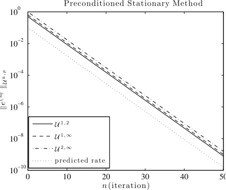
6.4. Numerical example for QCL-preconditioning. We now apply the QCL-preconditioned stationary iterative method to the QCF system with right-hand side (25), φ′′

F = 1, AF = 0.2, and the optimal valueα =αoptqcl,2,∞ (we note that Gid(αoptqcl,2,∞)

depends only on AF/φ′′F and N, but e(0) depends on AF and φ′′F independently). The

error for successive iterations in the _U1,2_,U1,∞ _andU2,∞_{-norms are displayed in Figure}

2. Even though our theory, in this case, predicts a perfect contractive behavior only in _U2,∞ _{and (partially) in U}1,2_{, we nevertheless observe perfect agreement with the}

optimal predicted rate also in the _U1,∞_{-norms. As a matter of fact, the parameters}

are chosen so that case (i) of Theorem 18 holds, that is, Gqcl(α) is nota contraction of

U1,∞_{. A possible explanation why we still observe this perfect asymptotic behavior is}

that the norm ofGqcl(α) is attained in a subspace that is never entered in this iterative

process. This is also supported by the fact that the exact solution is uniformly bounded in _U2,∞ _{asN, K → ∞, which is a simple consequence of Proposition 6.}

7. Preconditioning with QCE (P =Lqce_F ): Ghost-Force Correction

0 10 20 30 40 50 10−10

10−8 10−6 10−4 10−2 100

Preconditioned Stationary Metho d

n(iteration)

k

e

(

n

)k

U

k

,

p

U1,2

U1,∞

U2,∞

p red i cted rate

Figure 2. Error of the QCL-preconditioned linear stationary iterative method for the QCF system with N = 800, K = 32, φ′′

F = 1, AF = 0.2,

optimal value α = αqcl,2,_opt ∞, and right-hand side (25). In this case, the iteration matrix Gqcl(α) is not a contraction of U1,∞. Even though our

theory predicts a perfect contractive behavior only in _U2,∞_{, we observe}

perfect agreement with the optimal predicted rate also in the _U1,2 _and

U1,∞_-norms.

equations. The ghost force correction method in a quasi-static loading can thus be reduced to the question whether the iteration matrix

Gqce :=I−(LqceF )−1L qcf F

is a contraction. Due to the typical usage of the preconditioner Lqce_F in this case, we do not consider a step size α in this section. The purpose of the present section is (i) to investigate whether there exist function spaces in which Gqce is a contraction; and

(ii) to identify the range of the macroscopic strains F where Gqce is a contraction.

We begin by recalling the fundamental stability result for theLqce_F operator, Theorem 2:

inf

u∈U ku′

k_ℓ2

ε=1

hLqce_F u, u_i=AF +λKφ′′2F,

where λK ∼λ∗+O(e−cK) with λ∗ ≈0.6595. This result shows that the GFC iteration

must necessarily run into instabilities before the deformation reaches the critical strain

F∗

c. This is made precise in the following corollary which states that there is no norm

with respect to which Gqce is a contraction up to the critical strain F∗.

Corollary 19. Fix N and K, and let _{k · k}X be an arbitrary norm on the space U,

then, upon understanding Gqce as dependent on φ′′F and φ′′2F, we have

Despite this negative result, we may still be interested in the question of whether the GFC iteration is a contraction in “very stable regimes,” that is, for macroscopic strains which are far away from the critical strainF∗. Naturally, we are particularly interested

in the behavior as N _{→ ∞}, that is, we will investigate in which function spaces the operator norm of Gqce remains bounded away from one asN → ∞. Theorem 4 on the

unboundedness of Lqcf_F immediately provides us with the following negative answer.

Proposition 20. If 2_≤K _≤N/2, φ′′

2F 6= 0, and AF +λKφ′′2F >0, then

kGqcekU1,2 ∼N1/2 as N → ∞.

Proof. It is an easy exercise to show that, if AF +λKφ′′2F > 0, then the U1,2-norm is

equivalent to the norm induced by Lqce_F , that is,

C−1_ku_kU1,2 ≤ kuk_Lqce

F ≤ CkukU1 ,2.

Hence, we have _kGqcekU1,2 ≈ kG_qcek_Lqce

F and by the same argument as in the proof of

Proposition 13, and using again the uniform norm-equivalence, we can deduce that

Gqce

U1,2 ≈

Lqcf_{F L(U}1,2_,U−1,2₎±1∼N

1/2 _{as N}

→ ∞.

Since the operator (Lqce_F )−1_Lqcf

F is more complicated than that of (AFL)−1LqcfF , which

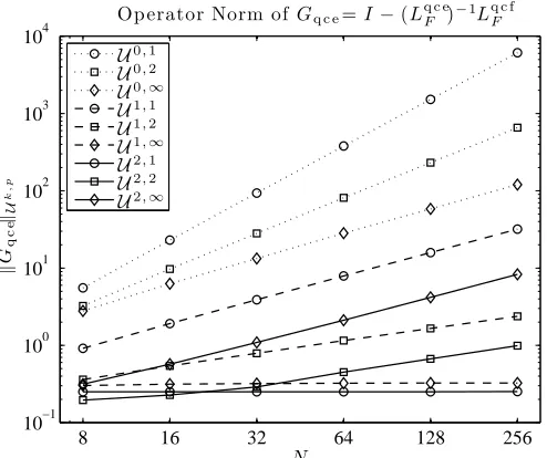
we analyzed in the previous section, we continue to investigate the contraction proper-ties of Gqce in various different norms in numerical experiments. In Figure 3, we plot

the operator norm of Gqce, in the function spaces

Uk,p, k = 0,1,2, p= 1,2,_∞,

against the system size N (see Appendix 8.3 for a description of how we compute kGqcekUk,p). This experiment is performed for A_F/φ′′_F = 0.8 which is at some distance

from the singularity of Lqce_F (we note that Gqce depends only on AF/φ′′F and N since

both (φ′′_F)−1Lqcf_F and (φ′′_F)−1Lqce_F depend only on AF/φ′′F and N). The experiments

suggests clearly that _kGqcekUk,p → ∞ as N → ∞ for all norms except for U1,∞ and

U2,1_.

Hence, in a second experiment, we investigate how _kGqcekU1,∞ and kG_qcek_U2,1

be-have, for fixed N and K, as AF +λKφ′′2F approaches zero. The results of this

exper-iment, which are are displayed in Figure 4, confirm the prediction of Corollary 19 that _kGqcekUk,p → ∞ as A_F + λ_Kφ′′_2F approaches zero. Indeed, they show that

kGqcekUk,p > 1 already much earlier, namely around a strain F where A_F ≈ 0.52

and AF +λKφ′′2F ≈0.44.

Our conclusion based on these analytical results and numerical experiments is that the GFC method is not universally reliable near the limit strain F∗, that is, under

8 16 32 64 128 256 10−1

100 101 102 103 104

N

k

Gq

c

e

kU

k

,

p

Operator Norm ofGq c e=I−(Lq c eF )

−1_Lq c f

F

U0,1

U0,2

U0,∞

U1,1

U1,2

U1,∞

U2,1

U2,2

U2,∞

Figure 3. Graphs of the operator norm _kGqcekUk,p, k = 0,1,2, p =

1,2,_∞, plotted against the number of atoms, N, with atomistic region size K =_⌈√N_{⌉ −}1, and AF/φ′′F = 0.8. (The graph for the U1,p-norms,

p = 1,_∞, are only estimates up to a factor of 1/2; cf. Appendix 8.3.) The graphs clearly indicate that_kGqcekUk,p → ∞asN → ∞in all spaces

except for _U1,∞ _{and U}2,1_.

shows at the very least that further investigations for more realistic model problems are required.

Conclusion

We proposed and studied linear stationary iterative solution methods for the QCF method with the goal of identifying iterative schemes that are efficient and reliable for all applied loads. We showed that, if the local QC operator is taken as the precondi-tioner, then the iteration is guaranteed to converge to the solution of the QCF system, up to the critical strain. What is interesting is that the choice of function space plays a crucial role in the efficiency of the iterative method. In_U2,∞_{, the convergence is always}

uniform in N and K, however, in _U1,∞ _{this is only true if the macroscopic strain is at}

some distance from the critical strain. This indicates that, in the presence of defects (that is, non-smooth solutions), the efficiency of a QCL-preconditioned method may be reduced. Further investigations for more realistic model problems are required to shed light on this issue.

We also showed that the popular GFC iteration must necessarily run into instabilities before the deformation reaches the critical strainF∗

c. Even for macroscopic strains that

are far lower than the critical strain F∗, we show thatkGqcekU1,2 ∼N1/2.We then give

numerical experiments that suggest that _kGqcekUk,p → ∞ as N → ∞ for all tested

The results presented in this paper demonstrate the challenge for the development of reliable and efficient iterative methods for force-based approximation methods. Further analysis and numerical experiments for two and three dimensional problems are needed to more fully assess the implications of the results in this paper for realistic materials applications.

0 0.2 0.4 0.6 0.8 1

10−2 10−1 100 101 102 103

AF

k

Gq

c

e

kU

k

,

p

Operator Norm ofGq c e=I−(Lq c eF )

−1_Lq c f F

AF

+

λ∗

φ

′

′

2

F

=

0 _U2,1

U1,∞_{, upper bd.}

U1,∞

, lower bd.

Figure 4. Graphs of the operator norm _kGqcekUk,p, (k, p) ∈

{(1,_∞),(2,1)_}, for fixed N = 256, K = 15, φ′′

F = 1, plotted against

AF. For the case U1,∞ only estimates are available and upper and lower

bounds are shown instead (cf. Appendix 8.3). The graphs confirm the result of Corollary 19 that _kGqcekUk,p → ∞ as A_F +λ_Kφ′′_2F →0.

More-over, they clearly indicate that _kGqcekUk,p > 1 already for strains F in

the region AF ≈ 0.5, which are much lower than the critical strain at

8. Appendix

8.1. Proof of Theorem 2. The purpose of this appendix is to prove the sharp stability result for the operator Lqce_F , formulated in Theorem 2. Using Formula (23) in [9] we obtain the following representation of Lqce_F ,

Lqce_F u, u =

( _−K−2 X

ℓ=−N+1

εAF|u′ℓ|2+ N

X

ℓ=K+3

εAF|u′ℓ|2

)

+

( _K−1 X

ℓ=−K+2

εAF|u′ℓ|2−ε2φ′′2F|u′′ℓ|2

)

+εn(AF −φ′′2F)(|u′−K+1|2+|uK′ |2) +AF(|u′−K|2+|u′K+1|2)

+ (AF +φ′′2F)(|u′−K−1|2+|u′K+2|2)

− 1 2ε

2_φ′′

2F(|u′′−K|2+|u′′−K−1|2+|u′′K|2+|u′′K+1|2)

o .

(29)

If φ′′

2F <0, then we can see from this decomposition that there is a loss of stability

at the interaction between atoms₋K₋2 and ₋K₋1 as well as between atomsK+ 1 and K+ 2. It is therefore natural to test this expression with a displacement ˆu defined by

ˆ

u′ ℓ =

    

1, ℓ=₋K₋1,

−1, ℓ=K+ 2,

0, otherwise.

From (29), we easily obtain

Lqce_F u,ˆ uˆ =AF + 1₂φ′′2F.

In particular, we see that, if AF + 1₂φ′′2F < 0, then L qce

F is indefinite. On the other

hand, it was shown in [8] that Lqce_F is positive definite provided AF +φ′′2F >0. (As a

matter of fact, the analysis in [8] is for periodic boundary conditions, however, since the Dirichlet displacement space is contained in the periodic displacement space the result is also valid for the present case.)

Thus, we have shown that

inf

u∈U ku′_k

ℓ2ε=1

Lqce_F u, u=AF +µφ′′2F, where 12 ≤µ≤1.

To conclude the proof of Theorem 2, we need to show that µdepends only on K and that the stated asymptotic result holds.

From (29) it follows that Lqce_F can be written in the form

where we identify u′ _{with the vector u}′ _{= (u}′

ℓ)Nℓ=−N+1 and whereH ∈R2N×2N. Writing

H =φ′′

FH1+φ′′2FH2,we can see that H1 = Id and that H2 has the entries

H2 =

            

. .. ... ...

1 2 1

1 2 1

1 3/2 1/2 1/2 3 1/2

1/2 9/2 0

0 4 0

0 4 0

. .. ... ...

            

Here, the row with entries [1, 3/2,1/2] denotes the Kth row (in the coordinates u′ k).

This form can be verified, for example, by appealing to (29). Let σ(A) denote the spectrum of a matrix A. Since, by assumption, φ′′

2F ≤0, the smallest eigenvalue of H

is given by

minσ(_H) =φ′′_F +φ′′_2Fmaxσ(_H2),

that is, we need to compute the largest eigenvalue ¯λ of _H2. Since H2ek = 4ek for

k = K + 3, K + 4, . . . and for K = ₋K ₋ 2,₋K ₋3, . . ., and since eigenvectors are orthogonal, we conclude that all other eigenvectors depend only on the submatrix describing the atomistic region and the interface. In particular, ¯λ depends only on K

but not on N. This proves the claim of Theorem 2 thatλK depends indeed only on K.

We thus consider the _{−K₋1, . . . , K + 2_}-submatrix ¯_H2, which has the form

¯ H2 =

           

9/2 1/2 1/2 3 1/2

1/2 3/2 1

1 2 1

. .. ... ...

1 2 1

1 3/2 1/2 1/2 3 1/2

1/2 9/2

            .

Letting ¯_H2ψ =λψ, then for ℓ=−K+ 2, . . . , K −1,

ψℓ−1+ 2ψℓ+ψℓ+1 =λψℓ,

and hence, ψ has the general form

ψℓ =azℓ+bz−ℓ, ℓ=−K+ 1, . . . , K,

leaving ψℓ undefined for ℓ ∈ {−K,−K −1, K+ 1, K + 2} for now, and where z,1/z

are the two roots of the polynomial

z2+ (2₋λ)z+ 1 = 0.

In particular, we have

z= (1

2λ−1) +

q (1