Integrating calculation and experiment : developing processes and tools for NMR crystallography of organic solids

A Thesis Submitted for the Degree of PhD at the University of Warwick

Permanent WRAP URL:

http://wrap.warwick.ac.uk/100468/

Copyright and reuse:

This thesis is made available online and is protected by original copyright.

Please scroll down to view the document itself.

Please refer to the repository record for this item for information to help you to cite it.

Our policy information is available from the repository home page.

M A E

G

NS I

T A T MOLEM

U N

IV

ER

SITAS WARWICEN SIS

Integrating Calculation and Experiment:

Developing Processes and Tools for NMR

Crystallography of Organic Solids

by

Miri Zilka

Thesis

Submitted to the University of Warwick

for the degree of

Doctor of Philosophy

Department of Chemistry

Contents

List of Tables iii

List of Figures iv

Acknowledgments v

Declarations vi

Abstract vii

Chapter 1 Introduction and Thesis Overview 1

Chapter 2 Background Information 5

2.1 Polymorphism . . . 5

2.1.1 Polymorphism in Pharmaceuticals . . . 6

2.2 Density Functional Theory . . . 7

2.3 Solid State Nuclear Magnetic Resonance Theory . . . 13

2.3.1 Magnetism . . . 13

2.3.2 Quantum Mechanical Description . . . 14

2.3.3 Density Operator . . . 16

2.3.4 Time Evolution of the Density Operator . . . 16

2.3.5 Solid-State NMR Interaction Hamiltonians . . . 17

2.3.6 J Coupling . . . 21

2.3.7 Quadrupole Interaction . . . 22

2.4 NMR experimental techniques and methods . . . 22

2.4.1 1D NMR Experiment . . . 22

2.4.2 Multi-Dimensional NMR Experiments . . . 23

2.4.3 The NMR spectrometer . . . 26

2.4.4 Magic Angle Spinning . . . 28

2.5 Computation of Magnetic Resonance Parameters . . . 34

2.5.1 GIPAW and CASTEP . . . 34

2.6 Crystal structure prediction . . . 42

2.7 NMR Crystallography . . . 44

Chapter 3 Ab-Initio Random Structure Searching of Organic Molec-ular Solids: Assessment and Validation Against Experimental Data 47

Chapter 4 Visualising packing interactions in solid-state NMR:

Con-cepts and applications 69

Chapter 5 An NMR Crystallography investigation of Furosemide 91

Chapter 6 Visualization and Processing of Computed Solid-State

NMR parameters: MagresView and MagresPython 106

List of Tables

2.1 Attributes that can vary between different polymorphs . . . 5

List of Figures

2.1 magnetic fields in a rotating frame of reference . . . 19

2.2 Effect of signal decay on spectral line shape . . . 23

2.3 A schematic pulse sequence of a 2D NMR experiment . . . 24

2.4 Processing required to achieve an absorption lineshape from a 2D NMR experiment . . . 26

2.5 Illustrative drawing of an NMR magnet . . . 27

2.6 Schematic diagram of an NMR spectrometer . . . 28

2.7 Sample in rotor aligned at the magic angle . . . 29

2.8 Pulse sequence and coherence transfer pathway diagram for a cross polarization (CP) experiment . . . 31

2.9 Pulse sequence and coherence transfer pathway diagrams for a 2D refocussed INEPT experiment . . . 32

2.10 Pulse sequence and coherence transfer pathway diagram for a 1_H -1_{H DQ experiment . . . . 32}

2.11 A schematic 1H -1H DQ spectrum . . . 33

Acknowledgments

I would like to thank my supervisor, Prof. Steven Brown, for the guidance, support

and flexibility he gave me over the course of my PhD. I am grateful to Prof. Alison

Rodgers for the opportunity to be a part of the CAS-IDP, and for always giving

me good advice. I would also like to acknowledge the funding from the European

Union, under a Marie Curie Initial Training Network, that enabled me to focus on

research work for the last four years. I would like to thank the MML group at Oxford

University for hosting me as a visiting researcher, and in particular Prof. Jonathan

Yates and Dr. Simone Sturniolo; Prof. Kenneth Harris and his group in Cardiff

University, in particular, Dr. Colan Hughes and Dr. Andrew Williams; Prof. Chris

Pickard. To my industrial liaison, Les Hughes; To all members of the solid-state

NMR group, and in particular those who assisted me in using the spectrometers.

To the rest of the Marie Curie CAS-IDP members: Maria Adobes Vidal, Erick

Ratamero, Jacopo Franco, Meropi Sklepari, Daniela Lobo, Alvin Teo, Roy Meyler,

Claudio Vallotto, Greg Walkowiak, Carl ¨Oster and Olga Nev, this journey wouldn’t

have been the same without you. Lastly, to my parents, who bravely endured the

Declarations

The work presented in this thesis is my own, except where stated otherwise in the

statement of contributions in page 46. The research was conducted under the

super-vision of Prof. Steven P. Brown at the University of Warwick between September

2013 and July 2017. This thesis has not been submitted for a degree at another

uni-versity. All of the results presented in this work, have been published or submitted

for publication:

Sturniolo, S., Green, T.F., Hanson, R.M., Zilka, M., Refson, K., Hodgkinson,

P., Brown, S.P. and Yates, J.R., 2016. Visualization and processing of computed

solid-state NMR parameters: MagresView and MagresPython. Solid state nuclear

magnetic resonance, 78, 64-70 (2016). (1)

Zilka, M., Dudenko D. V., Hughes, C. E., Williams, P. A., Sturniolo, S.,

Franks W. T., Pickard C. J., Yates, J.R., Harris, K. D. M. and Brown, S.P., 2017.

Ab-Initio Random Structure Searching of Organic Molecular Solids: Assessment

and Validation Against Experimental Data. Physical Chemistry Chemical Physics,

19, 25949-25960 (2017).(2)

Zilka, M., Sturniolo, S., Brown, S.P. and Yates, J.R, 2017. Visualising

pack-ing interactions in solid-state NMR: Concepts and applications. The Journal of

Chemical Physics 147, 144203 (2017).(3)

Zilka, M., Brown, S.P. and Yates, J.R, 2017. An NMR Crystallography

Abstract

The main goal of the work presented in this thesis is to develop and apply

com-putational tools for NMR crystallography, namely the combination of theoretical

and computational methods with experimental solid-state NMR and powder X-ray

diffraction. The Ab Initio Random Structure Searching (AIRSS) approach was

ap-plied to predict the structure of an organic solid, m-aminobenzoic acid (mABA).

Assessment of candidate structures was carried out against experimental powder

X-ray diffraction data and solid-state NMR data. A successful Le Bail refinement

and a good agreement between calculated and experimental NMR chemical shifts

was achieved for some of the lowest energy candidate structures, showing that two

polymorphs, forms-III and IV, had been identified. In further work a computational

framework to identify how the local environment affects the NMR shieldings has

been introduced. It is demonstrated that the majority of chemical shift variation

for protons comes from long-range current contributions whereas for heavier atoms

it is the short-range term that dominates. Magnetic Shielding Contributions Field

(MSCF) plots are introduced as a visualisation tool for identifying the contributions

to the magnetic shieldings from ring-currents and hydrogen-bonds. Next, an

experi-mental and theoretical analysis of the polymorphic active pharmaceutical ingredient

(API) furosemide is presented, employing the computational tools developed to

iden-tify local environment effects. Lastly, we highlight computational tools developed

List of Abbreviations

API Active Pharmaceutical Ingredient

NMR Nuclear Magnetic Resonance

BABA BAck-to-BAck

CP Cross Polarisation

DFT Density Functional Theory

DQ Double Quantum

DUMBO Decoupling Using Mind Boggling Optimisation

FID Free Induction Decay

FT Fourier Transform

GGA Generalised Gradient Approximation

GIPAW Gauge-Including Projector Augmented Waves

HK Hohenberg-Kohn

INEPT Insensitive Nuclei Enhanced by Polarisation Transfer

LDA Local Density Approximation

MAS Magic Angle Spinning

NICS Nucleus-Independent Chemical Shifts

NMR Nuclear Magnetic Resonance

PAS Principal Axis System

PAW Projector Augmented Waves

PBE Perdew-Bruke-Ernzerhof (GGA functional)

ppm parts per million

pXRD powder X-ray Diffraction

rf radio frequency

SQ Single Quantum

TMS Tetramethylsilane

Chapter 1

Introduction and Thesis

Overview

The aim of the work presented here is to contribute to the toolbox available within the field of NMR crystallography, aiding researchers who combine state of the art solid-state NMR experiments with ab initio calculations to investigate organic solids. In particular, there is a focus on an investigation of the packing interactions in a solid and their effect on magnetic shielding.

Solid-state NMR has developed significantly since the first NMR experiments

in the condensed phase, published independently by Purcell (4) and Bloch (5) in

1946. The most important development has been magic angle spinning (MAS), that was demonstrated to improve the resolution of spectra already in the late 1950s

(6) while cross polarization (CP), decoupling and 2D techniques also constitute

major advances. Nevertheless, solid-state NMR is an instrumental technique for solid structure investigation that is still in development today. Accompanying these experimental advances, there has been and continues to be considerable progress in the ab initio prediction of NMR parameters. The Gauge-Including Projector

Augmented Waves (GIPAW) method (7,8) enables calculation of NMR parameters

in the solid-state, with calculations possible on unit cells of up to _∼1000 atoms

for organic molecules. The consequence of this dual development is an increasing application of these methods in tandem. This work aims to improve the way these experimental and ab initio approaches work together, expanding the insights gained from calculations.

quan-tum theory of solid-state NMR, including the density operator description and the relevant interaction Hamiltonians is given. Practical considerations important for performing solid-state NMR experiments are also described, including MAS and a brief overview of the experiments used in this work. The method for calculating NMR parameters using DFT and the GIPAW is explained. Lastly, a short intro-duction to crystal structure prediction and NMR crystallography is presented.

Chapter 3 is a publication entitled “Ab Initio Random Structure Searching of Organic Molecular Solids: Assessment and Validation Against Experimental Data”. In this paper, the Ab Initio Random Structure Searching (AIRSS) approach is ap-plied for an organic compound m-aminobenzoic acid (mABA). The AIRSS method is an ab initio random searching method that uses DFT for geometry optimisation and energy ranking. AIRSS has been previously applied to inorganic materials and the

study of materials under very high pressure (9–14), however, this work is the first

example of using the AIRSS method to successfully predict experimentally observed structures of an organic molecule. An important focus of the work was assessing and validating the candidate structures produced using the AIRSS method with respect to experimental powder x-ray diffraction data and solid-state NMR data. mABA is a rigid molecule that has five known polymorphs. Form I is yet to be solved (this was a motivation in selecting mABA for the study), while published crystal structures exist for the other forms in which mABA is either zwitterionic (III & IV) or neutral (II & V). 600 candidate structures corresponding to unit cells with 4 zwitterionic molecular units and inversion symmetry were generated using AIRSS. In order to demonstrate the feasibility of using AIRSS in a search for a structure that cannot be solved from diffraction, yet where powder X-ray diffraction (pXRD) and solid-state MAS NMR data exists, the candidate structures were tested against pXRD and solid-state NMR data. The challenges in the comparison of ab initio structures to the experimental data are highlighted, in particular, it is demonstrated that

low-temperature pXRD data is required for a successful Le Bail refinement1 of DFT-D

geometry optimised structures. Structure solutions for both form III and form IV where found within the ten lowest energy candidate structures. Form III, the most thermodynamically stable form, was easiest to locate. The lowest energy candidate structure matched the known solution for form III. Note that form III only has one molecular unit in the asymmetric unit, reducing the effective degrees of freedom of the search. Metastable variants served an additional challenge in the case of form IV of mABA, where a successful fit to the pXRD data was only achieved after a

rotation of one of the CH3 group in the AIRSS structure was performed, leading to

the correct hydrogen-bonding arrangement and a more efficient three-dimensional packing.

Chapter 4 is a publication entitled “Visualising packing interactions in solid-state NMR: Concepts and applications”. Ab initio calculations have a proven ability to predict and assign experimental solid-state NMR spectra. However, such calcu-lations also have the potential to provide deeper information, such as why nuclei have specific NMR parameters and what this tells us about their local environ-ment. In this paper we introduce a theoretical framework to address these aims. We show how the magnetic shielding can be divided into short-range terms arising from current close to the nucleus in question, and to a long range contribution. An analysis of 71 molecular crystals shows us that the majority of change in the chemi-cal shift for protons comes from the long-range term, however for heavier atoms the short-range terms dominate. This is why protons are the most sensitive nuclei for NMR crystallography investigations of intermolecular interactions associated with different solid-state forms. In addition to a GIPAW calculation on the full unit cell, the NMR magnetic shieldings are calculated for a single molecule in a box, and the differences in magnetic shielding are analysed. A framework for calculating the Nuclear Independent Chemical Shift (NICS) is demonstrated, where a calcula-tion is performed on a unit cell containing neighbouring molecules but excludes the molecule of interest. We also introduced a quantity known as the Magnetic Shield-ing Contribution Field (MSCF). Plots of the MSCF highlight the regions of space responsible for the shielding of a particular atom. We show how the combination of these tools can be used to identify the contribution of ring currents due to aromatic motifs and hydrogen bonds on NMR chemical shifts. We apply this formalism to ex-amine the intermolecular interactions in a host-guest compound, a pharmaceutical polymorph and a co-crystal.

Chapter 5 details an experimental and computational investigation of the active pharmaceutical ingredient (API) furosemide. Furosemide is an organic com-pound of interest since, in addition to being produced as part of a medically valu-able drug, it exhibits polymorphism and low solubility in water. Previous work

on furosemide has focused on trying to understand (15) and solve (16, 17) the

focusing on the different hydrogen-bond motifs.

Chapter 2

Background Information

2.1

Polymorphism

A polymorph was defined by McCrone as a solid crystalline phase of a given

com-pound resulting from the possibility of at least two different arrangements of the molecules of that compound in the solid state (18). It is the ability of a solid to crystallise in more then one way, despite having the same chemical composition. Different polymorphs will exhibit different physical properties including thermo-dynamic stability, solubility, melting point and mechanical properties. A list of attributes that can vary between different polymorphs is presented in Table 2.1.

When crystallising from a liquid form, the production of a specific polymorph depends on the crystal nucleation and growth process, and may be affected by changing the solvent, temperature, humidity, or more advanced techniques such as high pressure treatment or sublimation (20,21).

Polymorphism is a common phenomena, with over a third of organic solids

reported to have more than a single solid form (22). However, compounds exhibiting

high polymorphism, i.e. more than three known polymorphs, are still uncommon, although this might be directly related to lack of effort in search attempts.

Cruz-Table 2.1: Attributes that can vary between different polymorphs (19).

Thermodynamic Kinetic Mechanical Packing Surface

Free Dissolution Hardness Density Surface

energy rate free energy

Heat Chemical Shear Conductivity Colour

capacity stability strength

Melting Rate of Compactability Morphology Sheen

Cabezaet al. (23) compared data from the Cambridge Structural Database (CSD) to data from solid form screens conducted at Hoffmann-La Roche and Eli Lilly and Company to discover that while in the CSD the ratio compounds exhibiting polymorphism is indeed a one in three, the screening test results produced a ratio of one in two. They further found that from more intensive screening efforts the ratio

rises to three in four, suggesting that McCrone was right in proclaiming that the

number of solid forms of a compound is proportional to the time and money spent investigating its crystallization (24).

The macroscopic differences exhibited by different polymorphs are due to the different inter-molecular interactions on the microscopic level. A change in the strength of hydrogen bonds for example, can change the solubility of the solid.

Differentiating between different polymorphs can be done by several exper-imental techniques, such as optical microscopy, thermal analysis, etc. Whenever possible, the preferred method for solving the crystal structure of different

poly-morphs is single crystal x-ray diffraction (21) (XRD). Solid-state NMR can also

differentiate between forms, since the magnetic shielding is sensitive to even small

changes in the inter-molecular arrangement (25). This is especially useful when a

single crystal cannot be produced, and the sample can only be analysed in

pow-der form (26–28). Different polymorphs will often have a different number of the

molecules in the asymmetric unit, that will directly effect the number of peaks observed in any recorded spectrum.

The first published investigation of polymorphism using solid-state NMR was

by Ripmeester in 1980 (29). Polymorphism has been investigated using13C and15N

experiments (25) due to the relative ease by which high resolution spectra can be

acquired. 1H solid-state experiments are very useful in the study of inter-molecular

interactions (30), that are fundamental to the investigation of polymorphism.

2.1.1 Polymorphism in Pharmaceuticals

The active pharmaceutical ingredient (API) is the therapeutic component of a drug. The API is usually mixed with excipients and can be administered as a tablet or suspended in liquid; a tablet is usually the preferred administration method. The drug development process is long and expensive, starting with around 5,000 initial compounds to reach one developed and approved drug within 7-10 years. Poly-morphism is tightly bound to the drug development process since it can potentially affect the stability, bioavillability (21), shelf lifetime and storage conditions of the drug, thus influencing its performance and quality (31–33).

between drug delivery problems and polymorphism. Polymorphism is still a key part of pharmaceutical research; in the drug discovery stage, when attempts are made to discover all polymorphs of an API, and in the manufacturing stage where control of the produced polymorph is critical (34,35). There is also a legal aspect to polymor-pism in an API. A patent is only valid for the polymorphs produced by the process registered in the patent. This was the basis of numerous court cases disputing intel-lectual propriety over poly morphs and other modifications (hydrates, solvates, etc.) of patented drugs. It is therefore of particular interest for pharmaceutical companies to have as thorough an understanding as possible of the polymorphic landscape of a drug in development.

In order to know about all polymorphs and other potential forms of interest (salts, co-crystal, hydrates, etc.) of an API, pharmaceutical companies invest in a

large scale solid form screening (36,37). This is an experimental process where the

API is exposed to a very large number (hundreds or even thousands) of different sets of crystallisation conditions. This process is both long and costly, however, perhaps the greatest difficulty is that there is no good way to know when to stop. There is a conflict of interests between the pressure to minimise the very high cost of the drug formulation process, with the potential consequences of failure to find a stable form before the drug reaches the market (38,39).

2.2

Density Functional Theory

Quantum Chemistry Concepts

The Schr¨odinger Equation

The Schr¨odinger equation is the starting point of quantum chemistry. Most quantum

chemical approaches attempt to solve, approximately, the time-independent, non-relativistic Schr¨odinger equation.

ˆ

HΨi(~r1, ~r2, ..., ~rN, ~R1, ~R2, ..., ~RM =EiΨi(~r1, ~r2, ..., ~rN, ~R1, ~R2, ..., ~RM) (2.1) ~ri and R~i are the positions of the ith electron and nucleus, respectively. ˆH is the

nuclei, without the presence of external fields:

ˆ

H =₋1 2

N

X

i=1

∇2i −

1 2 M X A=1 1

MA∇

2

A

| {z }

kinetic energy − N X i=1 M X A=1 ZA riA + N X i=1 N X j>i 1 rij + M X A=1 M X B>A ZAZB

RAB

| {z }

potential energy

(2.2) where atomic units are used and:

MA - mass of nucleus A

ZA- Charge of nucleus

rij - |r~i−r~j|interaction distance, RAB inter-nuclear distance

Ψi - wave function

Ei - Energy of the state Ψi

The first approximation we take for the Schr¨odinger equation is the

Born-Oppenheimer approximation. We fix the positions of the nuclei, making their po-tential energy zero. We can then define (in atomic units):

ˆ

Helec =−

1 2

N

X

i=1

∇2i − N X i=1 M X A=1 ZA riA + N X i=1 N X j>i 1

rij ≡

ˆ

T + ˆTN e+ ˆTee (2.3)

and the corresponding:

Enuc= M X A=1 M X B>A ZAZB

RAB

(2.4)

ˆ

HelecΨˆelec =EelecΨˆelec (2.5)

such that:

Etot =Eelec+Enuc (2.6)

The wave function is not an observable and it cannot be measured. The only physical representation of the wave function is that the square of the wave function:

|Ψi(~r1, ..., ~rN)|2d~r1...d~rN (2.7)

gives the probability that N electrons are found simultaneously in the volume given by d ~x1...d ~xN. If we integrate over all space, the result must be unity since all the

electrons must be found somewhere in space.

All electrons are fermions (spin=1₂). This means that the wave function must

both spatial and spin coordinates.

Ψi(~r1, ..., ~ri, ~rj, ..., ~rN) =−Ψi(~r1, ..., ~rj, ~ri, ..., ~rN) (2.8) The Variational Principle

Except for a few simple cases, it is not possible to solve the Schr¨odinger Equation

exactly. However, we can use the variational principle to systematically get closer

to the ground state Ψ0, and its corresponding ground state energy. The variational

principle states that the expectation value of a Hamiltonian operator, ˆH, for any

trial wave function Ψtrial will be higher than the energy of the ground state1:

hΨtrial|Hˆ|Ψtriali=Etrial≥E0=hΨ0|Hˆ|Ψ0i (2.9)

whereEtrial=E0 only if Ψtrial= Ψ0.

The problem is then reduced to the search of the wave function that gives us the lowest corresponding energy. In theory, to reach the ground state all we need to know is the number of electrons, and the location and charge of all nuclei.

The Electron Density

Keeping in mind the physical interpretation of the wave function, Ψ, we can define the electron density:

ρ(~r) =N

Z

...

Z

|Ψi(~x1, ..., ~xN)|2d~s1d~x2...d~xN (2.10)

ρ(~r) determines the probability of finding, within a given volume,N electrons, where

one has an arbitrary spin, due to integrating overd~s, and the rest N ₋1 have an

arbitrary position.

The electron density is an observable with a finite maximum, however, it has a ‘cusp’ like shape around the position of the nuclei. We can further extend this concept to define the pair density:

ρ2(~x1, ~x2) =N(N −1)

Z

...

Z

|Ψi(~x1, ~x2, ..., ~xN)|2d~x3...d~xN (2.11)

this gives the probability of finding two electrons with spinsσ1 andσ2in the volume

elements d ~x1 and d ~x2, with the rest of the electrons having arbitrary position and

spin. Since electrons are fermions, the probability of finding two electrons with

1_{Using Dirac notation, where ˆOis an operator andhOˆi=hΨ|Oˆ|Ψi=}R

...R

the same spin in the same position is zero. Hence, the position of one electron is correlated to the position of all the other electrons. We can define the ‘exchange

correlation hole’, which is the difference between the conditional probability2 _and

the uncorrelated probability:

hxc(~x1, ~x2) =

ρ2(~x1, ~x2)

ρ(~x1) −

ρ(~x2) =ρ(~x2)f(~x1, ~x2) (2.12)

The Hohenberg-Kohn Theorems

The First Hohenberg-Kohn Theorem:

This first theorem (40) states that the external potential Vext(~r) is (to within a

constant) a unique functional ofρ(~r); since, in turn Vext(~r) fixes Hˆ we see that the

full many particle ground state is a unique functional of ρ(~r).

This implies that two different potentials, Vext(~r) and Vext0 (~r), will never

result in the same ρ(~r). Hence the complete ground state energy is a functional of

the ground state electronic density.

E0[ρ0] =T[ρ0] +Eee[ρ0] +Ene[ρ0] (2.13)

We can divide the terms into components that are dependent on the specific system (N,RA,ZA) and ones that are not:

E0[ρ0] = T[ρ0] +Eee[ρ0]

| {z }

independent HK functional

+

Z

ρ0(~r)Vned~r

| {z }

system dependent

(2.14)

The Second Hohenberg-Kohn Theorem - Variational Principle:

The second HK theorem is the equivalent of the variational principle described by

Eqn. 2.9, but for the electron density. The theorem states that only the ρ(~r) that

represents the true ground state of the system, ρ0(~r), will deliver the ground state

energy.

hΨtrial|Hˆ|Ψtriali=T[ρtrial] +Vee[ρtrial] +

Z

ρtrial(~r)Vextd~r=E[ρtrial]≥ hΨ0|Hˆ|Ψ0i

(2.15)

2_{The probability of finding an electron atx~}

The Kohn-Sham Approach

We saw that the energy of the ground state can be reached by minimising the universal HK functional and the system dependent component. However, the ex-plicit form of the HK functional is the major challenge in DFT. The HK functional contains three contributions: kinetic energy, classical Coulomb interaction and the non-classical interaction:

FHK[ρ] =T[ρ] +J[ρ] +Vnc[ρ] (2.16)

The classical Coulomb interaction J[ρ] is the only known component in FHK[ρ].

The approach suggested by Kohn and Sham (41) is to calculate the kinetic energy

of a reference, fictitious, system of non-interacting electrons with the same density

ρ(~r) as the real system. The density is reformulated as a set of N single-particle

orthonormal functions,_|ψii, and the kinetic energy can now by calculated exactly:

Ts=−

1 2

N

X

i

hψi|∇2|ψii (2.17)

the difference between this solution to the real kinetic energy is added to the dif-ference between the classic potential and the non-classical one, introducing the exchange-correlation energy:

Exc[ρ] = (T[ρ]−Ts[ρ]) + (Eee[ρ]−J[ρ]) (2.18)

if the orbitals are chosen correctly, Exc[ρ] is usually small. This method computes

exactly as much information as possible, leaving only Exc[ρ] as an approximate

functional.

Minimising the Kohn-Sham functional results in the Kohn-Sham equations:

−1₂∇2+h Z ρ(r~

0₎

|~r₋~r0_|+Vxc(~r)−

M

X

A

ZA

|~r₋R~A| ψi(~r)

i

=εiψi(~r) (2.19)

this set of equations is the key to uniquely determining the orbitals on our non-interacting system such that the reference system will have the exact same density as the real one.

If we know the form ofVxcthese equations will result in the exact ground state

and energy. Unfortunately, this potential in unknown and must be approximated.

Vxc≡ δExc

δρ (2.20)

Exchange-Correlation Functionals

All known exchange-correlation functionals are approximate. The success of DFT is dependent on the success of the chosen exchange-correlation functional. Unfortu-nately, there is no known ‘one solution fits all’ and the functional needs to be chosen according to the desired application.

Although the real form of the exchange-correlation functional is inherently non-local, a local potential is computationally favourable. The simplest exchange-correlation functional is the Local-Density Approximation (LDA), suggested by

Kohn and Sham (41). LDA assumes that the exchange-correlation energy per

elec-tron, positioned at r is the same as an homogeneous electron gas with the same

density (per electron, at r):

Exc[ρ(~r)] =

Z

E_xchom[ρ(~r)]ρ(~r)d~r (2.21)

Ceperley and Alder (42) took the suggested LDA form, and found an

es-timate for the exchange-correlation functional by solving the ground state of the uniform electron gas using the Monte Carlo method. This estimate was then

pa-rameterised for use in DFT methods (43).

The LDA approach is usually not accurate enough for many chemical appli-cations. Typical problems with LDA includes over estimation of the binding energy and underestimation of the lattice parameters. The semi-local Generalised Gradient Approximation (GGA) includes a gradient correction to the electron density:

Exc[ρ(~r)] =

Z

E_xchom[ρ(~r),∇ρ(~r)]ρ(~r)d~r (2.22) This approximation is usually more accurate then LDA, but not always. Including the gradient can improve the total energy calculation since it reduces the error in bonding energy, but unlike LDA, GGA doesn’t have one universal form. The

Perdew-Bruke-Ernzerhof (PBE) functional (44) is one widely used parametrisation

of GGA.

assem-blies in biological material, van der Waals interactions are a key factor. One way of resolving this issue is through Van der Waals functionals. These have been

devel-oped (45–47), but unfortunately have not yet produced chemically accurate results

(48,49).

Another way to account for Van der Waals interactions is to use DFT-D schemes. DFT-D schemes correct the DFT energy with a semi-empirical disper-sion correction that accounts for long range forces that bind the molecules together by accounting for the London dispersion forces. The form of the pairwise energy correction due to the London dispersion forces is:

δE_ABdis = C6

R6 (2.23)

whereA and B are a pair of atoms. The difference between the DFT-D schemes is

in how the interatomic dispersion coefficients,C6, are calculated.

The scheme used in this work was suggested by Tkatchenko and Scheffler

(50) (denoted TS scheme). The TS scheme is a parameter-free method, where the

C6 coefficients are derived from the DFT electron density and reference data. This

is to account for the effect of the local environment of the atoms on the values of

theC6 coefficients. Other examples for DFT-D schemes are the Grimme dispersion

correction (G06 scheme) (51), OBS scheme (52) and the JCHS scheme (53).

Examples of DFT-D schemes applications, in particular TS and G06 schemes, are: study of the electronic structure and chemically bond of naphthalene and

an-thracene (54); side-stacking and electronic properties in thiophene–quinoxaline

poly-mers (55); polymorphism in methyl paraben (55); and hydrogen bonding and π-π

interactions in indomethacin and nicotinamide co-crystals (56)

2.3

Solid State Nuclear Magnetic Resonance Theory

The material presented in this section is based upon the theory and derivations that are presented in references (57–60).

2.3.1 Magnetism

The ratio between the induced magnetic moment, µ, and the applied

mag-netic fieldB0 is determined by χ, the magnetic susceptibility of the material:

µ_∝χB0 (2.24)

Materials with χ > 0 are paramagnetic, and will tend to align with the magnetic

field. Materials withχ <0 are diamagnetic, and attempt to reject the external field. Usually|χpara| |χdia|for bulk materials.

Magnetism has three microscopic sources: (i) electromagnetic currents, (ii) intrinsic magnetic moment of electrons, (iii) intrinsic magnetic moment of the nu-cleus. The nuclear magnetic moment is directly related to the spin of the nucleus:

µ=γI (2.25)

where γ is the gyromagnetic ratio, an intrinsic property of every nuclear isotope.

Most nuclei have aγ >0 while some nuclei (and the electron) have γ <0.

Spin Precession and the Larmor Frequency

The magnetic moment of a nucleus is aligned with the direction of the spin polar-ization (γ > 0) or opposite to it (γ < 0). The response of the spin polarisation to an external field is to precess around it - a cone shaped movement, keeping the angle between the spin and the magnetic field the same as it was when sample is first exposed to the field.

The frequency of the precession is the Larmor frequency:

ω0 =−γB0 (2.26)

The precession will either be clockwise or counter-clockwise, depending on the sign of the gyromagnetic ratio, γ.

2.3.2 Quantum Mechanical Description

The interaction energy of a single nucleus in an external static magnetic field, if the nucleus has a non-zero spin, is given by the Zeeman Hamiltonian:

ˆ

H =₋µˆ_·B0 (2.27)

where B0 is the external magnetic field and ˆµ is the nuclear magnetic moment

ˆ

µ=γIˆ (2.28)

ˆ

Iis the spin angular momentum operator andγthe gyromagnetic ratio, as previously

mentioned, an intrinsic property of the nucleus. If we define the ˆz axis in the

direction of the magnetic field, we can write Eqn. 2.28 as:

ˆ

Hz =−γIˆz·B0 =ω0Iˆz (2.29)

whereω0 is the Larmor frequency (from Eqn. 2.26).

Spin Angular Momentum Operator

The spin angular momentum operator measures the spin angular momentum, when acted on a wavefunction. We can define four operators: ˆIx, ˆIy, ˆIz and ˆI2, with the

following relationships:

ˆ

I2= ˆI_x2+ ˆI_y2+ ˆI_z2 [ ˆI2,Iˆz] = 0 [ ˆIx,Iˆy] =i¯hIˆz (2.30)

The eigenvalues of the ˆI2 _{and ˆI}

z operators are (in ¯hunits):

ˆ

I2|Ψi=l(l+ 1)|Ψi Iˆz|Ψi=m|Ψi (2.31)

wherem can range within the values₋l,₋l+ 1,...,+l. In the case ofl= 1₂, such as

1_{H and}13_{C nuclei,m can be−}1

2 or 12. The Zeeman eigenstates and eigenvalues for

a spin-half nucleus are:

ˆ

Hz| ↑i=

1

2ω0| ↑i Hˆz| ↓i=−

1

2ω0| ↓i (2.32)

commonly referred to as up (_{| ↑i}) and down (_{| ↓i}) states. A nucleus can also be in

a state of super-position of the eigenstates:

|Ψ_i=C↑| ↑i+C↓| ↓i (2.33)

|C↑|2 and |C↓|2 represent the probability of the spin to collapse to an up or down

2.3.3 Density Operator

When describing an ensemble of nuclei, it is useful to define the density operator:

ˆ

ρ=_|Ψ_ihΨ_| (2.34)

The over-bar notes an ensemble average of all the nuclear spin wavefunctions in the system (over-bar will be omitted from here onwards). For a system consisting of isolated half spin nuclei we can write ˆρ in a matrix representation:

ˆ

ρ= |C↑|

2 _C

↑C↓∗

C↓C_↑∗ |C↓|2 !

(2.35)

The density-matrix must be Hermitian, with the diagonal elements being the

ex-pectation values of ˆIz, which are always real and between [0,1]. The off-diagonal

elements are complex, and can be redefined as a real coefficient and a phase term:

C↓↑=a↓↑eiφ↓↑ (2.36)

inserting back into the density matrix:

ˆ

ρ= |a↑|

2 _a

↑a↓ei(φ↑−φ↓)

a↑a↓e−i(φ↑−φ↓) |a↓|2 !

(2.37)

The diagonal elements relate directly to the populations of the up and down states (the populations will be equal when not in the presence of a magnetic field). In a system of non-interacting spins with random phases, the off-diagonal terms average out to zero. The off-diagonal elements will only be non-zero in a system where a phase coherence exists between individual spins. This coherence can be created and detected in an NMR experiment.

2.3.4 Time Evolution of the Density Operator

To describe a spin system during an NMR experiment, one has to describe the

evolution of the density operator in time. While the Schr¨odinger equation describes

the time evolution of pure states, the Liouville-von Neumann equation determines the evolution in time of the density operator:

dρˆ(t)

Under the approximation that the Hamiltonian is constant in time (mostly valid for short periods of time) the solution to Eqn. 2.38 becomes:

ˆ

ρ(t) =e−Htˆ ρˆ(0)eHtˆ = ˆU(t)ˆρ(0) ˆU∗(t) (2.39) ˆ

U(t) is termed a ‘propagator’.

2.3.5 Solid-State NMR Interaction Hamiltonians

The Hamiltonian required to describe a solid-state NMR experiment, ˆHtotal, can be

divided into six different components:

ˆ

Htotal = ˆHZ+ ˆHrf + ˆHσ+ ˆHD+ ˆHJ + ˆHQ (2.40)

ˆ

HZ and ˆHrf represent the external interactions, Zeeman and radio-frequency,

re-spectively. The rest are internal interactions: magnetic shielding ( ˆHσ), The indirect

magnetic interaction between the nuclear spins and the external magnetic field; dipolar coupling ( ˆHD), direct magnetic between the nuclear spins; J-coupling ( ˆHJ),

indirect interaction of the nuclear spins through the electrons; and quadrupolar in-teraction ( ˆHQ), electric interaction between nuclei with spin > 1₂ and electric fields

within the sample.

Each of these can be expressed as an independent operator. Each opera-tor will have a special reference system - namely the principal axis system (PAS), where the operator will be diagonal, i.e., only the diagonal components are non-zero. Unfortunately, the different Hamiltonian components will often not have the same PAS.

Transferring between any two reference systems is achieved by a set of three rotations, defined by three Euler angles,α,β and γ:

R(α, β, γ) =Rz(α)Ry(β)Rz(γ) (2.41)

To describe such rotations, it is convenient to express the interaction operators using spherical tensors instead of Cartesian tensors:

ˆ

H =

2

X

j=0

j

X

m=−j

Only the coefficients,Ajm, change under rotation in space in the following way:

R(Ajm) = j

X

m0₌−j

(₋1)mD_m,mj 0(α, β, γ)Ajm0 (2.43)

whereD_m,mj 0 are known as Wigner rotation matrices.

High Field Approximation

The high field approximation, also known as the secular approximation, relies on the externally applied magnetic field being large enough to make the Zeeman interaction the dominant term. The approximation treats all other interactions as perturbations of the Zeeman Hamiltonian. This allows contributions only from terms that

com-mute with the Zeeman Hamiltonian. Specifically, only them= 0 tensor components

survive.

Zeeman Interaction

The Zeeman Hamiltonian is:

ˆ

HZ= ˆIZˆBˆ0=ω0Iˆz (2.44)

As previously described in Eqn. 2.29. The direction of ˆZ is the direction of the

magnetic field. Under all temperatures achievable in NMR experiments (more then a fraction above absolute zero), the density operator at thermal equilibrium, cor-responding to the start of an NMR experiment (assuming sufficient time for NMR relaxation to have occurred) will be:

ˆ

ρeq ∝Iˆz (2.45)

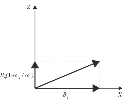
Radio frequency

B0 is not the only magnetic field applied in an NMR experiment (see Fig.2.1). An

oscillating, weaker field,B1(t) is introduced by a radio frequency (rf) pulse:

B1(t) = 2B1cos(ωrft+φ)ˆx (2.46)

B1(t) is generated by an oscillating current passing through a coil wrapped around

Z

X B0(1-ωrf / ω0)

B₁

Figure 2.1: The magnetic fields present in the rotating frame of reference (atωrf).

Figure adapted from ref. (61).

To consider the effect of both B0 and B1(t) on the density matrix, it is convenient

to define a resonance offset frequency Ω =ω0−ωrf.

Since unlikeB0,B1(t) is time-dependent, the radio frequency component of

the Hamiltonian is also time-dependent:

ˆ

Hrf =−γB1cos(ωrft) =ω1Iˆx (2.47)

withω1=−γB1 defined as the nutation frequency and for rf phaseφ= 0. In order

to remove the time dependency of the Hamiltonian, a transformation into a rotating reference system is required, specifically, a reference system that is rotating about the ˆz axis with aωrf frequency. B1(t) mixes the Zeeman states, but the eigenstates

remain the Zeeman eigenstates. The time-dependent propagation of the density matrix for a system of isolated spin-half nuclei under an on-resonant pulse is:

ˆ

ρ(t) =e−Hˆrft_ρˆ(0)eHˆrft₌ 1

2

cos(ω1t) isin(ω1t)

-isin(ω1t) -cos(ω1t)

!

(2.48)

For a starting point of thermal equilibrium (see Eqn. 2.45) we can see the effect of different pulses: a 90◦₍π

2) pulse makes diagonal terms (population) zero, and the

off-diagonal (coherence) non-zero, while a 180◦(π) pulse will cause the populations

to invert.

With a starting point of transverse magnetism created by a 90◦ _{pulse, the}

ˆ

ρ(t) = 1 2

0 e−iΩt

eiΩt 0

!

(2.49)

In an NMR experiment, the NMR signal corresponds to the induced current in a coil due to the precessing magnetisation. We can represent the recording of signal using quadruple detection (see section 2.4.1) to the operator [ ˆI+= ˆI−∗], where ˆI+= ˆIx+iIˆy

and ˆI− = ˆIx −iIˆy. Operating on the density operator will result in a real and

imaginary part (neglecting any losses due to relaxation):

T r( ˆI+ρˆ(t)) =

1

2(cos(Ωt) +isin(Ωt)) = 1 2e

iΩt _(2.50)

Magnetic Shielding

In the presence of a magnetic field, the orbit of electrons in a diamagnetic sample will induce a magnetic field opposing the applied external field. The effective magnetic field in the sample will vary depending on the electronic, i.e. chemical, environment. The Hamiltonian corresponding to this interaction is:

ˆ

Hσ =γIˆσB˜ 0 (2.51)

where ˜σ in the magnetic shielding tensor. In the spherical tensor representation

(see Eqn.2.42), the AP AS₀₀ component is rotationally invariant, and is proportional

to the sum of the diagonal values of the shielding tensor. However due to theAP AS

20

component, in an NMR spectrum of a powder (made of small crystals aligned in different orientations), we will get an anisotropic broadening of the spectral lines.

In an experiment, the measured quantity is the chemical shift, the relative

offset of the measured frequency from a reference frequency,ωref:

δiso=

ω−ωref ωref ×

106 (2.52)

The chemical shift is a dimensionless parameter that is expressed in parts per

mil-lions (ppm). Note that this value is independent of B0. 1H and 13C, are both

referenced against the compound TMS (Tetramethylsilane), for example. Other nuclei are referenced against other standard materials.

Dipolar Coupling

Hamiltonian of the dipolar interaction is:

ˆ

HD = ˆS1D˜Sˆ2 (2.53)

˜

D is a second-rank Cartesian tensor representing the interactions between ˆS1 and

ˆ

S2, the interacting spins. We can definebS1S2 (in units of rad

s ) as: bS1S2 =−

¯

hµ0

4π

γS1γS2

r3 (2.54)

whereµ0 is the permeability of space.

For a static experiment, in the spherical tensor representation, there is only a single component in the PAS:

ˆ

H_DP AS =√6bS1S2Tˆ20 (2.55)

and in the lab reference system for a static NMR experiment (see Eqn.2.43):

ALAB₂₀ =√6bS1S2

1 2(3 cos

2_(β)

−1) (2.56)

whereβ is the second Euler angle when rotating between the reference systems as

defined in Eqn. 2.41. In a powdered sample,β will vary between a range of values

due to the different crystallite orientations. As for the case of magnetic shielding, this will result in line broadening. In solution NMR these line broadening effects are eliminated by the rapid tumbling motion of the molecules, while in solid-state NMR, magic angle spinning (MAS) is used. Under MAS:

AM AS₂₀ =√6bS1S2

1 2(3 cos

2_θ

R−1)(3 cos2β−1). (2.57)

By choosingθRcorrectly, we can set AM AS20 to zero. MAS will be discussed further

in section 2.4.4, i.e. such that cosθR= √1₃.

2.3.6 J Coupling

of J-coupling was done in this work, however, the interaction is being utilized in experiments performed within this work, as further discussed in section 2.4.5.

2.3.7 Quadrupole Interaction

The Quadrupole interaction is the remaining internal interaction, however, it only affects nuclei with spin> 1₂, hence does not affect1H and13C nuclei studied in this work and will not be discussed here further.

2.4

NMR experimental techniques and methods

2.4.1 1D NMR Experiment

A basic one dimensional experiment consists of applying a 90◦ (π₂) pulse which

transfers the bulk magnetism the from the ˆz axis (the direction of B0) to the x

- y plane (the direction of B1). As mentioned in section 2.3.5, ωrf needs to be

equal or very close toω0. The signal detected is then mixed with the spectrometer

reference frequency,ωrf, such that the oscillation of the resonance offset frequency,

Ω, is observed.

Quadrature Detection

Signal detection is achieved using the quadrature detection technique - the signal is

detected in the x - y plane, with both a real and an imaginary component of the

NMR signal being recorded:

S(t) = (cos(pΩt)₋isin(pΩt))e−T₂t _=e−ipΩt_e−T₂t _{t≥0 (2.58)}

wherep is the coherence order. T2 is the time scale for the signal decay (so called

transverse relaxation), and is typically in the order of milliseconds for organic solids.

Note that for solids, T2 is much smaller then T1 (so called spin-lattice relaxation),

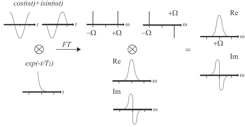
the characteristic time the system required to return to thermal equilibrium. The effects of the signal decay are demonstrated in Fig. 2.2.

It is helpful to view the signal in the frequency domain:

S(ω) =A(ω)−iD(ω) = T

−1 2

T₂−2+ (ω−Ω)2

| {z }

absorptive

−i (ω−Ω)

T₂−2+ (ω−Ω)2

| {z }

dispersive

+Ω −Ω

+Ω

−Ω

cos(ωt)+isin(ωt)

exp(-t/T2)

FT

=

Im

+Ω

Re

Im

ω ω

t t

t

ω

ω

ω

ω

Figure 2.2: The effect of multiplying the signal (cos(ωt) +isin(ωt)) by the decaying

functione−t/T2 _{after a Fourier transform. The result is two line shapes, absorptive}

(Re) and dispersive (Im). Figure adapted from ref. (61).

The different lineshapes are illustrated in Fig. 2.2. BothA(ω) andD(ω) are centred

at Ω, however, A(ω) is maximal at ω = Ω while D(ω = Ω) = 0. Since it is

not practically possible to just disregardD(ω), the most desirable lineshape of the

spectrum is achieved by adjusting the phase between the real and imaginary parts of the linear combination. This is referred to as ‘phasing’ the spectrum.

In practise the spectrometer uses a discrete Fourier Transform with the

spec-tral width, SW, constrained by the inverse of the time between data points for

acquisition (dwell time).

The only coherences directly detectable in a NMR experiment are single

quantum coherences (p=±1). Higher order coherences can be observed indirectly,

which is discussed in the section below.

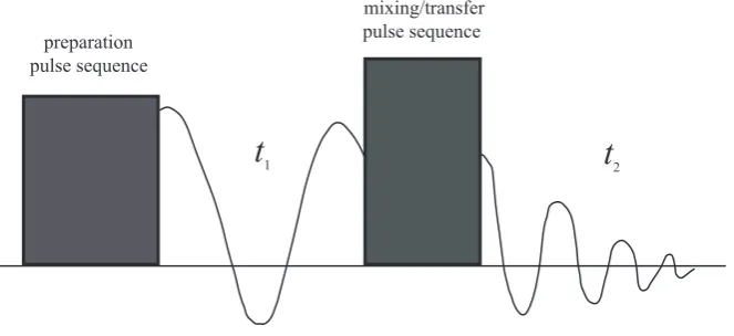
2.4.2 Multi-Dimensional NMR Experiments

indirect dimension(s), before the coherences with order of ∆p=_±1 can be observed directly. In a two-dimensional (or higher) experiment, non-observable coherences are transferred into observable coherence for detection or heteronuclear correlation can be established. Fig. 2.3 presents a schematic pulse sequence illustrating this process: an initial rf pulse (preparation sequence) brings the system to an

out-of-equilibrium state; afterwards, the system is allowed to evolve for a duration of t1;

the transfer pulse then transfers then-order coherences into₋1 coherences that are

recorded duringt2.

preparation pulse sequence

mixing/transfer pulse sequence

t

t

Figure 2.3: A schematic pulse sequence of a general 2D NMR experiment. Figure adapted from ref. (61).

The amplitude or the phase of the recorded signal is modulated according

to the evolution duringt1. By repeating the experiment while varyingt1, a second

dimension is generated. One dimension will contain information from the ₋1

co-herences, and second from the n-order coherences. Selecting the desired order of

coherence is achieved by phase cycling, as discussed in the section below.

The interpretation of a 2D spectrum is a correlation map. A peak at (ω1, ω2)

indicates that during t1 there was an n-order coherence with a ω1 frequency, that

transformed into a−1 coherence with a frequency of ω2.

This principle can be extended to higher-dimension experiments, but since these are not presented in this work, they will not be discussed further.

Phase Cycling

The first golden rule of phase cycling is the following(62): If the phase of a pulse is changed by φ, a coherence undergoing a change in coherence level of ∆p

acquires a phase shift of∆p_·∆φ. In a single phase cycle, the experiment is repeated

N times while incrementing the phase of the selected pulse(s) by 360_No, and letting

the receiver phase follow appropriately. Note that a receiver phase of 180o means

multiplying the signal by -1, while 90o _{means switching the real and imaginary}

parts. The result is that a pathway that corresponds to a change in coherence order of ∆p±n·N,where nis an integer, will prevail while others will be eliminated.

Table 2.2 demonstrates how a desired pathway 0_→ 2_→ +1 _{→ −}1, can be

selected while an undesirable pathway, 0 _{→ −}1 _→ +1 _{→ −}1, is eliminated using

phase cycling.

Table 2.2: Choosing a desired coherence pathway and eliminating an undesired one

using phase cycling. Table adapted from ref. (61)

cycle step pulse phase coherence phase receiver phase phase relative to receiver

desired pathway 0→2→+1→ −1

1 0◦ 0◦ 0◦ 0◦

2 90◦ _-180◦ ₁₈₀◦ ₀◦

3 180◦ _-360◦ ₀◦ ₀◦

4 270◦ -540◦ 180◦ 0◦

undesired pathway 0→ −1→+1→ −1

1 0◦ 0◦ 0◦ 0◦

2 90◦ 90◦ 180◦ 90◦

3 180◦ ₁₈₀◦ ₀◦ ₁₈₀◦

4 270◦ 270◦ 180◦ 270◦

Quadrature Detection for Two-Dimensional Experiments

A flowchart describing the quadrature detection process for 2D experiments is pre-sented in Fig. 2.4. In a 2D experiment, it is vital that the sin(ω1t1) and cos(ω1t1)

components, corresponding to the first dimension, can be recorded separately, in addition to recording sin(ω2t2) and cos(ω2t2), corresponding to the second

dimen-sion, separately. If recorded together, the Fourier transform of the recorded signal will be:

eiω1t1_eiω2t2 _→(A

1A2−D1D2) +i(A1D2−D1A2) (2.60)

whereA1 =A(ω1) and similarly for A2, D1 and D2. In this case, the lineshape of

the real part will bephase-twisted.

ex-periment is altered so that the coherence is phase shifted by 90◦ ₍π

2) between the

experiments. This is achieved by shifting the phases of the preparation pulses by

π

2∆n, where ∆nis the difference in coherence order from the start of the experiment

to after the preparation pulse.

C1cos(ω1t1)C2exp(iω2t2) C1sin(ω1t1)C2exp(iω2t2)

C1cos(ω1t1)(A2+iD2) C1sin(ω1t1)(A2+iD2)

C1cos(ω1t1)A2 C1sin(ω1t1)A2

iC1sin(ω1t1)A2

C1(cos(ω1t1)+isin(ω1t1))A2

(A1+iD1)A2

A1A2

FT in t2

keep real part

multiply by i

add

FT in t1

keep real part

Figure 2.4: A flowchart describing the processing required to achieve a pure

absorp-tion lineshape from a 2D NMR experiment. Figure adapted from ref. (61).

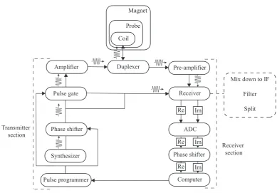
2.4.3 The NMR spectrometer

Figure 2.5: An illustrative drawing of an NMR magnet with a probe and a sample inside.

heart of the magnet, a Nb-Sn coil, is immersed in a bath of liquid He, surrounded

in a liquid N2 reservoir, to keep the magnet at the correct running temperature.

The sample itself is inserted into a probe, a separate device which is inserted into the spectrometer with the sample at the position of most homogeneous magnetic field. Inside the probe the sample is irradiated with rf waves, and the induced signal due to precession of magnetisation from the sample is detected. MAS probes spin the sample according to the desired limit and the capability of the probe. Probes usually also have temperature control features as well.

The signal detected in the coil inside the probe head is that of the carrier

frequency plus the offset frequency,ω0+ Ω. The signal is then amplified in the

pre-amplifier. Afterwards, the signal is mixed down to oscillate around an intermediate

frequency, ωIF + Ω. Mixing the frequency down means that the spectrometer is

required to deal with a smaller range of frequencies. This is done by mixing the

signal with a spectrometer generated frequency of ω0−ωIF and a filter that only

selects the component oscillating aroundωIF.

The real and imaginary parts of the signal are then separated by routing two

Coil Probe

Magnet

Duplexer Pre-amplifier

Receiver

Mix down to IF

Filter

Split

ADC

Phase shifter

Computer Pulse programmer

Amplifier

Pulse gate

Synthesizer Phase shifter

Im Re

Im Re

Im Re Transmitter

section

Receiver section

Figure 2.6: A schematic diagram of an NMR spectrometer, showing the console,

magnet and probe. Adapted form ref. (57).

The complex signal is then converted to a digital signal in the ‘analogue to digital converter’ (ADC).

2.4.4 Magic Angle Spinning

In solid-state NMR experiments, the sample studied is usually a powdered sample, containing many crystallites in different orientations. Both magnetic shielding and

dipolar interaction have a term with angular dependence of (3 cos2_{β−1) (see Eqn.}

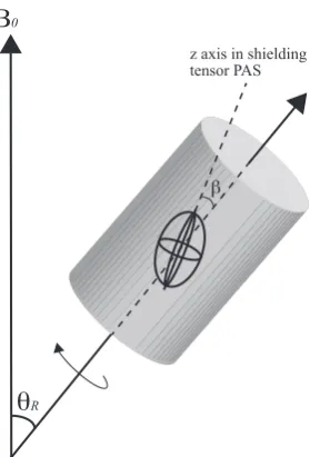
2.56) whereβis the angle between the ˆzaxis of the shielding tensor PAS as defined in Eqn. 2.41 and the rotation axis (see Fig.2.7). As previously mentioned, in solution-state NMR these are averaged out due to the rapid tumbling motion of the molecules while in liquid state.

If the sample is spun at an angle ofθR relative to the ˆzaxis in the lab frame

it can be shown that, averaged over one rotor period:

h3 cos2θ₋1_i= 1 2(3 cos

2_θ

θ

Β

z axis in shielding tensor PAS

β

Figure 2.7: Rotation of a sample at the ‘magic angle’, θR, during an MAS

experi-ment. β is the angle between the ˆz axis of the shielding tensor PAS as defined in

Eqn. 2.41.

IfθRis set to 54.74◦, the term in Eqn. 2.61 averages to zero. Spinning side-bands

The spinning frequency should ideally be fast in comparison to the anisotropy of the interaction that we are trying to eliminate. The chemical shift anisotropy is

proportional to the external applied field, B0, therefore faster spinning is useful

when a larger magnetic field is applied. If the MAS frequency is less then the linebroadening, ‘spinning side-bands’ are observed. These are sharp lines, separated by the spinning frequency, centred around the line of the isotropic chemical shift.

At the moment, commercial probes above 100 kHz are available, however, they come at the cost of a smaller rotor, hence less sample volume (for example, Bruker makes a 111 kHz probe for a 0.7 mm rotor).

2.4.5 Experiments Used in the Presented Work

Cross Polarization

Cross polarization (CP) is typically used to observe less abundant nuclei, such as

13_{C, by transferring magnetization from a more abundant nuclei, typically,}1_{H. The}

and combined with a lower gyromagnetic ratio, it is difficult to observe directly for

two main reasons: first, low signal-to-noise ratio; second, long T1 relaxation time

due to lack of strong homo-nuclear dipolar interactions. 1_{H, on the other hand,}

is about 99.99% naturally abundant, giving a strong signal while suffering from

lack of resolution due to strong homonuclear1H-1H dipolar coupling. Since the1H

relaxation time is usually much shorter then13_{C, it is not required to wait until the}

13_{C nuclear spins return to equilibrium between experiments, allowing a more rapid}

signal acquisition.

In the CP technique, i.e. application of rf irradiation on both nuclei simul-taneously, the magnetisation is usually transferred from a nucleus with a higher

gyromagnetic ratio (usually1H), to a nucleus with a lower gyromagnetic ratio. The

optimal enhancement gained isγ1

γ2 (4 for

1_{H and}13_{C). To achieve the transfer of}

mag-netisation, the amplitude of the pulses must be set such that the Hartmann-Hahn condition is satisfied (63):

γ1B1(S1) =γ2B1(S2) (2.62)

and with MAS:

γ1B1(S1) =γ2B1(S2)±nνR (2.63)

whereνRis the MAS spinning frequency, and γ1 andγ2 are the gyromagnetic ratios

of S1 and S2 nuclei, respectively. An efficient CP transfer is achieved by using a

ramped pulse on the 1_{H channel such that the rf nutation frequency is increased}

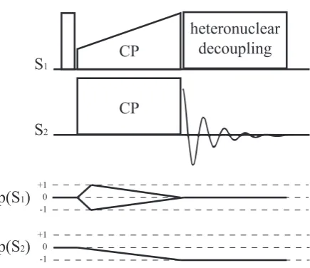
gradually during the contact time pulses (64). See Fig. 2.8.

The efficiency of the transfer depends upon the strength of the dipolar inter-action. This means that in a CP spectrum, the intensity of the peak is not purely an indication of the number of nuclear species, since it is weighted by a dependence on the corresponding carbon atoms’ proximity to hydrogens.

C-H correlation experiment - INEPT

In the INEPT (insensitive nuclei enhanced by polarization transfer) (65, 66)

ex-periment, magnetization is transferred between nuclei of bonded atoms. Similar to the one-dimensional CP experiment, the maximal gain in sensitivity is the ratio of

gyromagnetic ratios: γ1

γ2, which is 4 for

1_{H and} 13_{C. The difference is that in an}

INEPT experiment, a J coupling is used to transfer the magnetization rather than a dipolar coupling.

CP

CP

heteronuclear decoupling S1

S2

p(S1) +1

0 -1

+1 0 -1

p(S2)

Figure 2.8: Pulse sequence and coherence transfer pathway diagram for a cross

polarization (CP) experiment. The magnetization is transferred from the high γ

nuclei,S1 to the lower γ nuclei, S2.

by adding homonuclear decoupling that, in addition to MAS, reduces the1H dipolar

interaction (67). Only bonded13C -1H pairs will appear in the spectrum, and when

used with a shortτ period, the experiment is selective only to pairs linked by a single bond. A refocused INEPT pulse sequence and coherence diagram is presented in

Fig. 2.9. Transverse magnetization is allowed to evolve during t1. As seen in Fig.

2.9, the heteronuclear transfer occurs via the second π₂ pulse on the 1_{H channel.}

The second heteronuclear spin-echo block (τ0 - π - τ0) refocuses the signal which

results in in-phase peaks, that do not cancel each other out. In solid-state NMR

experiments,τ and τ0 _{are optimized for each sample.}

DUMBO Homonuclear Decoupling Scheme

DUMBO (decoupling using mind boggling optimization) (68,69) scheme uses

on-resonance rf pulses to apply homonuclear decoupling. A series of pulses with the same frequency are applied with a varying phase. This is based on the BLEW-12

scheme (70). eDUMBO-122 (71) is an optimized version of fast MAS.

1_{H -} 1_{H Double Quantum Experiment}

1_{H double quantum (DQ) correlation experiments are used to identify inter-molecular}

proximities between 1_{H pairs. The experiment probes both inter-molecular and}

eDUMBO θ t1 π 2 π -θ eDUMBO θ -θ

π 2 eDUMBO θ π -θ eDUMBO TPPM

π π₂ π

+1 0 -1 +1 0 -1

τ τ τ' τ' t2

p( H)

p( C) 1

13

Figure 2.9: Pulse sequence and coherence transfer pathway diagrams for a 2D13C

- 1H refocussed INEPT experiment using eDUMBO-122 homonuclear decoupling.

Figure is adapted from ref. (67).

other.

DQ excitation

p +10 -1 +2

-2

t1

x -x y -y

τ τ τR _n τ τ τR _n DQ reconversion

x -x y -y

t2

Figure 2.10: Pulse sequence and coherence transfer pathway diagram for a1H -1H

DQ experiment using BABA dipolar recoupling.

All the1H -1H DQ experiments presented in this work use the Back-to-Back

(BABA) dipolar recoupling scheme (72, 73). The scheme is used to excite and

reconvert DQ coherence (∆p = _±2). The basic BaBa scheme consists of four 90◦

pulses and two periods of free evolution per rotor period (τR). Repeating the BaBa

cycle over several rotor periods corresponds to longer dipolar recoupling times. A schematic pulse sequence and coherence transfer pathway diagram is presented in

It was demonstrated that under MAS, due to time reversal symmetry, a

sim-ple 90 -τ - 90 pulse sequence will result in a disruptive interference that eliminates

the signal after a single rotor period (τR). In the BaBa sequence, a 90◦ phase shift

of the two pulses on the second half of the sequence is introduced to overcome this obstacle (74–76).

The result of the experiment is a two-dimensional spectrum, where peaks

only appear for coupled pairs. Usually, only peaks for pairs of1H nuclei closer then

3.5 ˚A will appear in the spectrum (74). A schematic diagram of the spectrum is

presented in Fig. 2.11.

δ

δ

δ

+δ

δ

+δ

B

_B'

A

< 3.5Å

Figure 2.11: A schematic spectrum for a1H -1H DQ experiment, showing a

corre-lation map for 2 nuclei that are separated by less than 3.5 ˚A. In this simple case,

Aand B represent different nuclei, and B0 _{is a symmetry copy ofB. The distances}

betweenAandB,AandB0 andB andB0are all under 3.5 ˚A. In the SQ dimension,

the peaks appear at the isotropic chemical shift, while in the DQ dimension, they are at the sum of the chemical shifts.

If homonuclear decoupling is used, the chemical shielding is also scaled in

both the 1H SQ and DQ dimensions of the spectrum. In order to calibrate the

2.5

Computation of Magnetic Resonance Parameters

2.5.1 GIPAW and CASTEP

Infinite Periodic Crystals

While macroscopic crystals are not actually infinitely large, they do contain a very large number of repeating units, the unit cell, such that most atoms within the crystal effectively ‘feel’ the environment of an infinite crystal.

Performing a simulation on all of the electrons in a real sample is impossible, but luckily, also unnecessary due to the periodic nature of the crystal. We can exploit the transitional symmetry that exists in all crystalline materials and focus a calculation on a single unit cell. By applying periodic boundary conditions we are in fact calculating the values for an infinite periodic crystal.

Bloch’s Theorem

Calculating an infinite crystal from a single unit cell is possible because of Bloch’s theorem: If the potentialV(~r) is periodic on a lattice such that V(~r) =V(~r+a~i)

where ai is a lattice vector, then we can write the eigenstate of the single-particle

Hamiltonian as:

ψ_~k(~r) =ei~k·~ru_~k(~r) (2.64)

where u_~k(~r) has the same periodicity as V(~r): u_~k(~r) = u_~k(~r+a~i) for all lattice

vectorsai.

These are called ‘Bloch states’ and are labelled by their crystal momentum

~k. Unique values of ~k only exist within one unit cell of the reciprocal lattice, or

within the 1st Brillouin Zone (also known as the Wigner-Seitz cell in the reciprocal lattice). Fig. 2.12 gives a schematic representation of the unit cell, the reciprocal cell and the k-point sampling grid.

Planewave Basis Set

When attempting to solve the Kohn-Sham equations Eqn. (2.19) numerically, we are presented with the choice of a basis set for the Khon-Sham eigenstates. Choosing a planewave basis set, we can express the eigenstates as follows:

ψ_~k(~r) =X

i

L

(a)

_(b)

(c)

L 2π

(d)

Figure 2.12: Figure adapted form Ref. (77). (a) The unit cell in real space, with

the lattice shown in black. (b) The darker atoms are the unique atoms that must be included in the calculation. (c) The reciprocal cell, with the gamma point (the origin) indicated by a circle and the first Brillouin zone marked by a dashed line (d) The first Brillouin zone divided by a uniform grid of sampling points, though because of symmetry considerations, only the grid points in the triangle need to be calculated explicitly.

whereGi are the reciprocal lattice vectors. c_~k(G~i) are determined by solving Eqn.

(2.19).

There are many possible choices for a basis set, however, planewaves are naturally periodic and converge systematically as a function of the size of the basis, making them very suitable as a basis set for the Kohn-Sham eigenstates in crystalline solids.

Since the solution is numerical, we must limit the size of the basis set. This

is achieved by only summing overG~i contained within a sphere with a given radius

such that:

¯

h2|~k+G~|2

2m ≤Ecut (2.66)

The larger the cut-off energy,Ecut, is, the more accurate the solution will be, but