Online Full Text

Abstract—In this paper we present a visual odometry system for agricultural field robots that is not sensitive to uneven terrain. A stereo camera system is mounted perpendicular to the ground and height and traveled distance are calculated using normalized cross correlation. A method for evaluating the system is developed, where flower boxes containing representative surfaces are placed in a metal-working lathe. The cameras are mounted on the carriage which can be positioned manually with 0.1 mm accuracy. Images are captured every 10 mm over 700 mm. The tests are performed on eight different surfaces representing real world situations. The resulting error is less than 0.6% of traveled distance on surfaces where the maximum height variation is measured to 96 mm. The variance is measured for eight test runs, total 5.6 m, to 0.040 mm. This accuracy is sufficient for crop-scale agricultural operations.

Index Terms—Agricultural applications, Image processing, Mobile robot localization, Visual odometry.

I. INTRODUCTION

There are a many sensors that can be used for localization of an outdoor mobile agricultural robot. Common ones are wheel encoders, GPS, inertial measurement unit (IMU) and machine vision [1],[2]. Usually these are used in combination to provide a global position estimate. This position can be fairly accurate if expensive sensors are used.

On an agricultural robot, the global position does not always have to be that accurate when operating on a field. More important are the robot’s position relative the crops, if the aim is agricultural operation on crop-scale. This requires an ability to navigate locally at high precision [3]. An example is a robot having a camera sensor detecting and classifying crops, and an active tool performing individual plant operations out of sight of the camera, Fig. 1. The position measurement of the tool relative the camera has to be done with high accuracy, to perform close to crop operations. Further there is an advantage to keep a tool, like a mechanical weed tool, far away from the camera sensor to prevent dust and soil from covering the lens. In these situations there is a need for a non-contact sensor that can measure short distances with high precision.

Manuscript received July 2, 2008. This work was supported by University of Skövde.

S. Ericson is with the University of Skövde, Box 408, 54128 Skövde, Sweden (phone: +46 500 448509; fax: +46 500 448599; e-mail: [email protected]).

B. Åstrand is with the Halmstad University, Box 823, 30118 Halmstad, Sweden (e-mail: [email protected]).

Figure 1. Weed-robot on a sugar beet field [3].

A good GPS sensor (RTK-GPS) can provide as low as 1 cm error of horizontal position [4], but only under good conditions. Error sources are the numbers of satellites visible, signal multi-path and dropouts. This position is also global, and not directly related to the crops measured in the images from the camera.

A camera sensor and an algorithm comparing consecutive frames, also known as visual odometry, can provide this non-contact measurement. There are different methods to determine the position. Work on visual odometry has been done with both mono and stereo cameras and with cameras mounted at different angle to the ground [5]-[9].

The feasibility of a visual odometer system has been shown in [5], where high slip terrain on Mars surface makes it hard to navigate using wheel encoders. Since there is no system for global positioning such as the GPS system on Mars, the visual odometry has become a critical vehicle safety system. A stereo camera setup is used and Harris corners are detected as features, which are matched and tracked using RANSAC with least square estimator for outlier rejection.

Other work using forward looking stereo cameras for visual odometry are presented in [6]. Reported error was less than 3% without filtering and less than 1% in combination with other sensors (IMU).

In [7] different algorithms are evaluated for visual odometry using a single camera pointing perpendicular to the ground. This method assumed planar ground, which makes this solution sensitive to changes in the height of the camera above the ground. Reported error was 0.3% on planar ground and up to 7.7% on uneven grass due to calibration error.

Similar work has been done in [8] where a sensor used in

Visual Odometry System for Agricultural Field

Robots

optical mouse is adapted for an outdoor environment on a mobile robot. The camera and image processing is incorporated in a chip which gives a frame rate at 6 kHz. Two sensors are used for calculating heading and traveled distance, but each sensor assumes planar ground. This assumption also makes the system sensitive to tilt of the robot where one sensor is closer and the other is further away from the ground. Reported error after calibration on a straight planar surface was 0.3%.

In [9] two cameras are used, also mounted on each side of the robot. Each camera are measuring distance as a mono camera using phase correlation technique and the system are analyzed from an odometry perspective obtaining position and heading. The error reported was similar to wheel odometry.

The objective with this paper is to demonstrate the feasibility of a system for high precision visual odometry in agricultural field environment.

The contribution of this paper is a visual odometry system for uneven terrain and an evaluation of the feasibility by experiments on real field situations.

II. MATERIAL AND METHOD A. Method

The major drawback of mono camera system, including systems based on optical mice chips, is the assumption that the ground is flat. Usually the clearance between the camera and the surface is held constant by mechanical design, as in an optical mouse. This method is not suitable for an outdoor mobile robot on an agricultural field. A stereo camera setup and epipolar geometry provides a measurement of the distance between the camera and to the point evaluated. This is used to compensate for the errors caused by differences in heights. This method will also provide an easy way to calibrate the system. Only one stereo pair is analyzed so the heading of the robot is assumed to be known. Methods for obtaining direction using by omnidirecitonal camera is explained in [10] or by a row following system in [3].

The cameras are mounted perpendicular to the ground according to Fig. 2. This mounting will provide maximum translation between images and hence no projection of images to a ground plane is needed. Further the position is only measured in 2D.

Figure 2. Camera configuration on robot. The 2D distance is measured with respect to a plane parallel to the camera lenses.

The use of stereo camera on a moving robot requires good synchronization. Any delay between the images will generate an error if the robot is moving. Speeds in the direction though the camera centers will be detected as a change of height and speed in the other direction will make an offset of the epipolar line. Therefore the cameras are synchronized by a hardware trigger. To reduce any errors caused by synchronization, the pair of stereo cameras should be mounted perpendicular to the main heading of the robot as shown in Fig 1, since translation in the other direction only occur when the wheel slips.

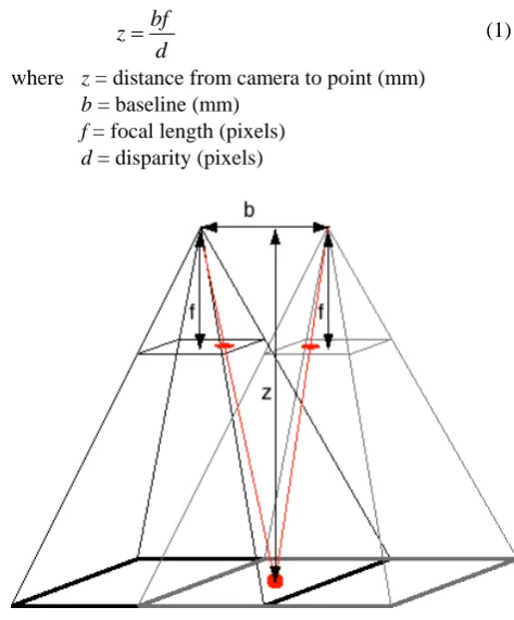
Considering a stereo camera setup [11] according to Fig. 3, the distance to a point can be calculated using (1).

d bf

z= (1)

where z = distance from camera to point (mm)

b = baseline (mm)

f = focal length (pixels)

d = disparity (pixels)

Figure 3. Camera model.

B. Matching

As shown in [7] several methods exist for analyzing the translation between consecutive images. If feature points are extracted, then some kind of matching algorithm is required to calculate translation. In [12] Harris corners are extracted and in the matching are performed with normalized cross correlation over an 11x11 pixel neighborhood. Usually normalized cross correlation is used on small regions. Two reasons are less computational cost and fewer problems caused by different projections of the images. The perpendicular mounting of the cameras and selection of a lens with low distortion reduces these problems.

k

k-1

Left image

Right image

d

d

d

d

Matching window

Frame Frame

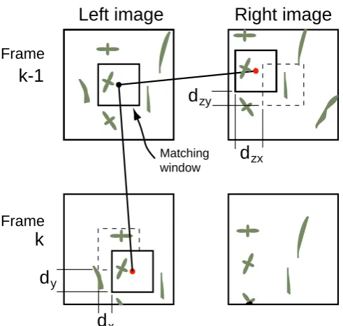
Figure 4. Method of matching images for height and distance. k is frame number and d is disparity.

The disparity dzx depends on the height to the object which is of interest. Disparity dzy depends on camera alignment and camera synchronization. In a calibrated system this disparity should be zero, which means that the search area in the right image can be limited. Disparity (dx,dy) is the measurement of traveled distance.

Images with different heights in the same matching window are expected in a field environment. Stereo matching of a region will average the heights over that region. The same region is then used for matching distance, as shown in Fig. 4. This means that the height is the same for both matches. Therefore is the distance traveled is height independent.

From (1) the height can be calculated as:

zx

d f b

z= ⋅ (2)

Assuming that the height are equal for the stereo match and distance match the relation can be written as:

zx

x d

f b d

f x

z= ⋅ = ⋅ (3)

which gives:

) ( ) ( ) (

k d

b k k

zx

⋅ =dx

x (4)

where x(k) = traveled distance (x,y) (mm) dx(k) = disparities (dx,dy) (pixels)

The relation between maximum speed, camera parameters and pixel resolution are shown in (5).

f d z fps

vy y

max , min max

,

⋅ ⋅

= (5)

where vy, max = maximum speed in y direction(m/s)

fps = framerate (frames/sec)

C. Validation Gate

A validation gate is implemented to remove outliers. Region matching by normalized cross correlation suffer from the aperture problem, which occurs when the values of the pixels does not change in the direction of the motion [14]. In these situations the similarity image will provide a bank with exactly the same values on the top. One way to determine the most probable match is to create a score function based on distance to previous match and peak height. In the case of a bank with lots of point with similar values to the point on the top closest to previous match will be selected. If no peak is found at all, the validation gate selects the point with highest value in the similarity image.

There are usually several peaks in the similarity image when an outlier occurs. If all peaks where selected for evaluation even a small peak at the same point as previous match will get a high score, since the distance is zero. Therefore only peaks within a certain range from the maximum peak value are selected.

D. Experimental setup

A method of testing the proposed system was developed. Two USB cameras, MV BlueFOX-120aC, are mounted on the carriage of a metalworking lathe, as shown in Fig. 5. Then they can be moved linearly in one direction over approximately one meter with high precision. This setup provides a ground truth, something that usually is difficult to obtain in an outdoor field environment. A realistic surface is created by using flower boxes with typical crops, in this case sugar beet. These boxes can be fit into the lathe.

Figure 5. Test setup in lathe with cameras and flower box (grass and sugar beet).

The carriage is positioned on the start position at one end of the flower box. Image pairs are captured while the carriage is moved to the other end of the flower box. This gives a total distance of 700 mm in y-direction for each test. The space in x-direction is so limited that no tests were possible to make in this direction.

stereo cameras is acquired and the carriage is moved 10mm for acquiring next pair. The cameras are not moved while the images are captured, which will eliminate errors from camera synchronization and motion blur. By capturing images at constant distance, the speed will be constant and the position for each image will be known. A drawback of this method is that the variance in the manual positioning each 10 mm will be included in the result. The accuracy of the positioning is approximately 0.1 mm. The mean error will be small due to the long distance.

For the evaluation of the dynamic performance, a constant frame rate is used. The carriage is moved a specified distance, in this case 700 mm, with various speeds. That means this test will include both synchronization error and motion blur, but there will not be a reference for each image, only for the entire distance. All tests are done by recording data and the analyses are performed offline using Matlab.

III. EXPERIMENTS

Three different tests are performed; first on a reference track to calibrate the system, second on various real surfaces consisting of soil and sugar beets for variance calculation, and third for evaluating the dynamic performance.

The first reference track is flat and the other consists of linear slopes and some blocks according to Fig. 6. The height to the reference level is measured to z = 453 mm, and the height of the camera is 96 mm which gives a clearance of 357mm from the ground to the lens.

Figure 6. Height profile of reference track 2.

The texture is artificial with light background and dark dots. Fig. 7 shows the surface texture of the two reference tracks.

(a) Reference track 1 (b) Reference track 2

Figure 7. Texture of the two reference tracks. The image of reference track 2 is taken at one steep slope, which causes the color shift.

There are eight tracks prepared for tests on real surfaces. The texture is selected to cover different difficulties. Four of them are on flat surface, which means there are no intentional slopes made. These tracks are created by flattening the soil by hand. The other four are with uneven surface. These tracks are created by shaping the profile with approximately three

bigger holes. The maximum height difference on a track is approximately 100 mm. Three main textures are selected; sugar beet in soil, sugar beet in soil with weed, sugar beet in grass. There are also one track on flat soil and one on uneven soil with weed.

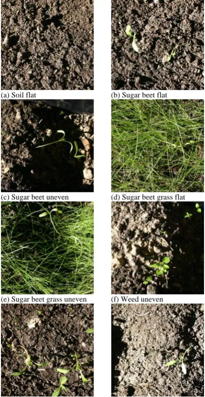
The different test surfaces are shown in Fig. 8 taken with a high resolution camera, and Fig. 9 as seen from the cameras used for image processing.

(a) Soil flat (b) Sugar beet flat

(c) Sugar beet uneven (d) Sugar beet grass flat

(e) Sugar beet grass uneven (f) Weed uneven

(g) Sugar beet weed flat (h) Sugar beet weed uneven

Figure 8. Texture examples of the eight flower boxes using high resolution camera.

(c) Sugar beet uneven (d) Sugar beet grass flat

(e) Sugar beet grass uneven (f) Weed uneven

(g) Sugar beet weed flat (h) Sugar beet weed uneven

Figure 9. Texture examples of the eight flower boxes using BlueFOX camera. Image size 200×200 pixels for illustration of texture.

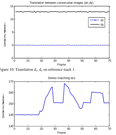
The result from the tests on the reference track is shown in Fig. 10 and Fig. 11. It can be seen that the translations measured on reference track 1 are constant with some noise, and on the reference track 2 the stereo disparity follows the height profile of the track, according to Fig. 5.

0 10 20 30 40 50 60 70

-5 0 5 10 15

Translation between consecutive images (dx,dy)

Dis p ari t y (pix els )

Frame

dx dy

Figure 10. Translation dx, dy on reference track 1.

0 10 20 30 40 50 60 70

130 140 150 160 170

Stereo matching dzx

Dis p ari t y (p ix els )

Frame Figure 11. Disparity dzx on reference track 2

The tests on the eight tracks contains 70 image pairs each, resulting in a total distance of 700 mm for each test. The data are analyzed using a 51×51 pixel window corresponding to approximate 40×40 mm at height 450 mm. The error and variance of the measurement in driving direction of robot (y- direction) are presented in Table I.

In total 5.6 m on various surfaces using 560 stereo pairs, the variance is measured to 0.040 mm which means 99.7% of the measurements are found within 0.60 mm. The variance measured includes both the manual positioning of the lathe carriage, and the error of the visual odometry system. Fig. 12 shows plots for the disparities measured and calculated traveled distance for the test on sugar beet sawed on uneven soil.

0 10 20 30 40 50 60 70

-5 0 5 10 15 20

Translation between consecutive images (dx,dy)

Dis p ari t y (pix els )

Frame

dx dy

(a) Measured translation

0 10 20 30 40 50 60 70

130 140 150 160 170

180 Stereo matching dzx

Dis p ari t y (p ix els )

Frame

(b) Measured stereo disparity TABLE I RESULT OF TESTS ON 700MM

Test

Measured distance

y (mm)

Error (%)

Varian ce (mm)

Height variation

(mm)

a. Soil flat 702.5 0.36 0.0084 14

b. Sugar beet flat 695.9 -0.59 0.057 24

c. Sugar beet uneven

699.9 -0.018 0.013 77

d. Sugar beet grass flat

702.1 0.31 0.024 27

e. Sugar beet grass uneven

704.1 0.590 0.042 55

f. Weed uneven 702.0 0.29 0.045 96

g. Sugar beet weed flat

699.2 -0.11 0.087 39

h. Sugar beet weed uneven

0 10 20 30 40 50 60 70 -2

0 2 4 6 8 10 12

Traveled distance (x,y)

Dis ta nc e ( m m )

Frame

x y

(c) Calculated distance traveled

Figure 12. Example of measured translation, disparity and calculated distance. These plots are from the test on sugar beet on uneven soil.

The height dependence of the translation disparity (dy) can clearly be seen by comparing it to the stereo disparity (dzx)

The dynamic test is performed on one surface only, sugar beet with weed on uneven soil, Fig. 8h. The frame rate is set to 5 Hz and the carriage is moved 10 times over the same distance with various speeds. The total distance for each test is 700 mm. The result is shown in Table II. There where several frame that where missing in these tests due to capturing problem. That error has been compensated for by selecting the correct image pairs for analyze.

Fig. 13 shows a plot of the disparity representing the height with respect to the estimated position for all 10 test runs.

-100 0 100 200 300 400 500 600 700 800

110 120 130 140 150 160 170 180

Dynamic performance, height vs position

Dis p ari t y d z x (pix els )

y (mm)

Figure 13. Result of 10 test run on sugar beet with weed on uneven ground.

IV. CONCLUSION

The system shows a small error, below 0.6% for these tests. The highest variance for a single run is found on the test “sugar beet flat”. It is measured to 0.057 mm. The accuracy is still sufficient for crop-scale agricultural operations. The error for the dynamic test is less than 0.23% which indicates that the error depends more on the texture and height profile than of the speed.

The error and variance is very dependent on outliers, which usually occurs when the images contains shadows or the texture is poor. In these situations the similarity image contains several peaks, where the highest ones are candidates to be the selected match. Shadows can be reduced and texture can be enhanced by improving the illumination. The system is also sensitive to missing frames. However, these are both easy to detect and to compensate for, for instants by double the search area in next image.

Further work will include real-time implementation of algorithm on a robot with steering control, using either row-following system or omnidirectional camera. The camera mounting and illumination has to be improved to reduce the number of outliers. Further more tests have to be

done in real environment to evaluate the system on a robot. REFERENCES

[1] J.F. Reid, Q. Zhang, N. Noguchi, M. Dickson, Agricultural automatic guidance research in North America, Computers and Electronics in Agriculture 25, 2000, 155-167

[2] T. Hauge, J.AMarchant, N.D. Tillet, Ground based sensing systems for autonomous agricultural vehicles, Computers and Electronics in Agriculture 25, 2000, 11-28

[3] B. Åstrand, A.J. Baerveldt, Vision-based perception for an agricultural mobile robot for mechanical weed control, Autonomous Robots 13, 2002, 21–35.

[4] S. Gan-Mor, R.L. Clark, B.L. Upchurch, Implement lateral position accuracy under RTK-GPS tractor guidance, Computers and Electronics in Agriculture 59, 2007, 31-38

[5] M. Maimone, Y. Cheng, L. Mattheis, Two years of visual odometry on the mars exploration rovers, Journal of Field Robotics 24(3), 2007, 169-186

[6] M. Agrawal, K.Konolige, Rough terrain Visual odometry, Proceedings of the International Conference on Advanced Robotics (ICAR), Jeju island, South Korea, 2007

[7] S. Ericson, B. Åstrand, Algorithms for Visual Odometry in Outdoor Field Environment, Proceedings of 13th IASTED International Conference Robotics and Applications, Würzburg, Germany, 2007, 287-292

[8] W. Seemann, K.D. Kuhnert, Localisation for an outdoor robot by optically measuring the ground movement, Proceedings of 13th IASTED International Conference Robotics and Applications, Würzburg, Germany, 2007, 113-118

[9] M. Zaman, High resolution relative localisation using two cameras, Robotics and Autonomous Systems 55, 2007, 685-692

[10] P. Corke, D. Strelow, S. Singh, Omnidirectional visual odometry for a planetary rover. IEEE/RSJ International Conference on Intelligent Robots and Systems (IROS). Sendai, Japan, 2004, 4007- 4012 [11] E. Trucco, A. Verri, Introductory techniques for 3-D computer vision,

(Prentice-Hall Inc. Upper Saddle River, New Jersey, USA)

[12] Z. Zhu, T. Oskiper, O. Naroditsky, S. Samarasekera, H.S. Sawhney, R. Kumar, An Improved Stereo-based Visual Odometry System, Performance Metrics for Intelligent Systems Workshop,USA, 2006, 149-156

[13] J. Westerweel, Effect on sensor geometry on the performance of PIV interrogation. Proceedings of the 9th International Symposium on Applications of Laser Techniques to fluid Mechanics, Lisbon, Portugal, 1998, 1-2

[14] B. Jähne, Digital image processing. (Berlin: Springer, 2002). TABLE II

RESULT OF DYNAMIC TESTS ON SUGAR BEET WEED UNEVEN 700MM

Test Measured

distance y (mm) Error (%)

1 698.9 -0.15

2 698.4 -0.23

3 699.0 -0.15

4 699.3 -0.098

5 698.9 -0.16

6 698.7 -0.19

7 699.1 -0.14

8 699.7 -0.046

9 699.7 -0.046