Adaptive Semi supervised Learning for Cross domain Sentiment Classification

3467

Adaptive Semi-supervised Learning for Cross-domain

Sentiment Classification

Ruidan He†‡_{, Wee Sun Lee}†_{, Hwee Tou Ng}†_{, and Daniel Dahlmeier}‡

†_{Department of Computer Science, National University of Singapore}

‡_{SAP Innovation Center Singapore}

†_{{ruidanhe,leews,nght}@comp.nus.edu.sg} ‡_{[email protected]}

Abstract

We consider the cross-domain sentiment clas-sification problem, where a sentiment classi-fier is to be learned from a source domain and to be generalized to a target domain. Our ap-proach explicitly minimizes the distance be-tween the source and the target instances in an embedded feature space. With the differ-ence between source and target minimized, we then exploit additional information from the target domain by consolidating the idea of semi-supervised learning, for which, we jointly employ two regularizations – entropy minimization and self-ensemble bootstrapping – to incorporate the unlabeled target data for classifier refinement. Our experimental results demonstrate that the proposed approach can better leverage unlabeled data from the target domain and achieve substantial improvements over baseline methods in various experimental settings.

1 Introduction

In practice, it is often difficult and costly to anno-tate sufficient training data for diverse application domains on-the-fly. We may have sufficient la-beled data in an existing domain (called the source domain), but very few or no labeled data in a new domain (called the target domain). This issue has motivated research on cross-domain sentiment classification, where knowledge in the source do-main is transferred to the target dodo-main in order to alleviate the required labeling effort.

One key challenge of domain adaptation is that data in the source and target domains are drawn from different distributions. Thus, adaptation per-formance will decline with an increase in distribu-tion difference. Specifically, in sentiment analy-sis, reviews of different products have different vo-cabulary. For instance, restaurants reviews would contain opinion words such as “tender”, “tasty”, or

“undercooked” and movie reviews would contain “thrilling”, “horrific”, or “hilarious”. The intersec-tion between these two sets of opinion words could be small which makes domain adaptation difficult. Several techniques have been proposed for ad-dressing the problem of domain shifting. The aim is to bridge the source and target domains by learning domain-invariant feature representa-tions so that a classifier trained on a source do-main can be adapted to another target dodo-main. In cross-domain sentiment classification, many works (Blitzer et al.,2007;Pan et al.,2010;Zhou et al.,2015;Wu and Huang,2016;Yu and Jiang,

2016) utilize a key intuition that domain-specific features could be aligned with the help of domain-invariant features (pivot features). For instance, “hilarious” and “tasty” could be aligned as both of them are relevant to “good”.

Despite their promising results, these works share two major limitations. First, they highly de-pend on the heuristic selection of pivot features, which may be sensitive to different applications. Thus the learned new representations may not ef-fectively reduce the domain difference. Further-more, these works only utilize the unlabeled tar-get data for representation learning while the sen-timent classifier was solely trained on the source domain. There have not been many studies on ex-ploiting unlabeled target data for refining the clas-sifier, even though it may contain beneficial infor-mation. How to effectively leverage unlabeled tar-get data still remains an important challenge for domain adaptation.

unla-beled data, assuming the domain distance can be effectively reduced through domain-invariant rep-resentation learning. Specifically, the proposed approach jointly performs feature adaptation and semi-supervised learning in a multi-task learning setting. For feature adaptation, it explicitly mini-mizes the distance between the encoded represen-tations of the two domains. On this basis, two semi-supervised regularizations – entropy mini-mization and self-ensemble bootstrapping – are jointly employed to exploit unlabeled target data for classifier refinement.

We evaluate our method rigorously under multi-ple experimental settings by taking label distribu-tion and corpus size into consideradistribu-tion. The re-sults show that our model is able to obtain sig-nificant improvements over strong baselines. We also demonstrate through a series of analysis that the proposed method benefits greatly from incor-porating unlabeled target data via semi-supervised learning, which is consistent with our motivation. Our datasets and source code can be obtained from

https://github.com/ruidan/DAS.

2 Related Work

Domain Adaptation: The majority of feature adaptation methods for sentiment analysis rely on a key intuition that even though certain opinion words are completely distinct for each domain, they can be aligned if they have high correlation with some domain-invariant opinion words (pivot words) such as “excellent” or “terrible”. Blitzer et al. (2007) proposed a method based on struc-tural correspondence learning (SCL), which uses pivot feature prediction to induce a projected fea-ture space that works well for both the source and the target domains. The pivot words are selected in a way to cover common domain-invariant opinion words. Subsequent research aims to better align the domain-specific words (Pan et al., 2010; He et al., 2011;Wu and Huang, 2016) such that the domain discrepancy could be reduced. More re-cently, Yu and Jiang (2016) borrow the idea of pivot feature prediction from SCL and extend it to a neural network-based solution with auxiliary tasks. In their experiment, substantial improve-ment over SCL has been observed due to the use of real-valued word embeddings. Unsupervised representation learning with deep neural networks (DNN) such as denoising autoencoders has also been explored for feature adaptation (Glorot et al.,

2011; Chen et al., 2012; Yang and Eisenstein,

2014). It has been shown that DNNs could learn transferable representations that disentangle the underlying factors of variation behind data sam-ples.

Although the aforementioned methods aim to reduce the domain discrepancy, they do not explic-itly minimize the distance between distributions, and some of them highly rely on the selection of pivot features. In our method, we formally con-struct an objective for this purpose. Similar ideas have been explored in many computer vision prob-lems, where the representations of the underlying domains are encouraged to be similar through ex-plicit objectives (Tzeng et al., 2014; Ganin and Lempitsky,2015;Long et al.,2015;Zhuang et al.,

2015;Long et al.,2017) such as maximum mean discrepancy (MMD) (Gretton et al.,2012). In NLP tasks, Li et al. (2017) and Chen et al. (2017) both proposed using adversarial training framework for reducing domain difference. In their model, a sub-network is added as a domain discriminator while deep features are learned to confuse the discrim-inator. The feature adaptation component in our model shares similar intuition with MMD and ad-versary training. We will show a detailed compar-ison with them in our experiments.

Semi-supervised Learning: We attempt to treat domain adaptation as a semi-supervised learning task by considering the target instances as unla-beled data. Some efforts have been initiated on transfer learning from unlabeled data (Dai et al.,

2007; Jiang and Zhai, 2007; Wu et al., 2009). In our model, we reduce the domain discrep-ancy by feature adaptation, and thereafter adopt semi-supervised learning techniques to learn from unlabeled data. Primarily motivated by ( Grand-valet and Bengio, 2004) and (Laine and Aila,

2017), we employed entropy minimization and self-ensemble bootstrapping as regularizations to incorporate unlabeled data. Our experimental re-sults show that both methods are effective when jointly trained with the feature adaptation objec-tive, which confirms to our motivation.

3 Model Description

3.1 Notations and Model Overview

We conduct most of our experiments under an un-supervised domain adaptation setting, where we have no labeled data from the target domain. Con-sider two setsDsandDt.Ds={x(is),y

(s)

from the source domain withnslabeled examples,

whereyi 2RC is a one-hot vector representation

of sentiment label and C denotes the number of classes.Dt={x(_it)}|n_i=1t is from the target domain

withntunlabeled examples.N =ns+ntdenotes

the total number of training documents including both labeled and unlabeled1_{. We aim to learn a}

sentiment classifier fromDsandDtsuch that the

classifier would work well on the target domain. We also present some results under a setting where we assume that a small number of labeled target examples are available (see Figure3).

For the proposed model, we denoteG parame-terized by✓gas a neural-based feature encoder that

maps documents from both domains to a shared feature space, and F parameterized by ✓f as a

fully connected layer with softmax activation serv-ing as the sentiment classifier. We aim to learn fea-ture representations that are domain-invariant and at the same time discriminative on both domains, thus we simultaneously consider three factors in our objective: (1) minimize the classification error on the labeled source examples; (2) minimize the domain discrepancy; and (3) leverage unlabeled data via semi-supervised learning.

Suppose we already have the encoded features of documents {⇠(_is,t) = G(x_i(s,t);✓g)}|Ni=1 (see

Section4.1), the objective function for purpose (1) is thus the cross entropy loss on the labeled source examples

L= 1

ns ns

X

i=1

C

X

j=1

y(_is)(j) log ˜y(_is)(j) (1)

wherey˜(_is)=F(⇠(_is);✓f)denotes the predicted

la-bel distribution. In the following subsections, we will explain how to perform feature adaptation and domain adaptive semi-supervised learning in de-tails for purpose (2) and (3) respectively.

3.2 Feature Adaptation

Unlike prior works (Blitzer et al., 2007; Yu and Jiang,2016), our method does not attempt to align domain-specific words through pivot words. In our preliminary experiments, we found that word embeddings pre-trained on a large corpus are able to adequately capture this information. As we will

1_{Note that unlabeled source examples can also be}

in-cluded for training. In that case,N =ns+nt+ns0 where

ns0denotes the number of unlabeled source examples. This

corresponds to our experimental setting 2. For simplicity, we only considernsandntin our description.

later show in our experiments, even without adap-tation, a naive neural network classifier with pre-trained word embeddings can already achieve rea-sonably good results.

We attempt to explicitly minimize the distance between the source and target feature represen-tations ({⇠(_is)_}|ns

i=1 and {⇠ (t)

i }ni=1t ). A few

meth-ods from literature can be applied such as Maxi-mum Mean Discrepancy (MMD) (Gretton et al.,

2012) or adversary training (Li et al.,2017;Chen et al., 2017). The main idea of MMD is to esti-mate the distance between two distributions as the distance between sample means of the projected embeddings in Hilbert space. MMD is implicitly computed through a characteristic kernel, which is used to ensure that the sample mean is injective, leading to the MMD being zero if and only if the distributions are identical. In our implementation, we skip the mapping procedure induced by a char-acteristic kernel for simplifying the computation and learning. We simply estimate the distribution distance as the distance between the sample means in the current embedding space. Although this ap-proximation cannot preserve all statistical features of the underlying distributions, we find it performs comparably to MMD on our problem. The follow-ing equations formally describe the feature adap-tation lossJ:

J =KL(gs||gt) +KL(gt||gs) (2)

g0_s= 1

ns ns

X

i=1

⇠(_is), gs= g

0

s

kg0

sk1 (3)

g0_t= 1

nt nt

X

i=1

⇠_i(t), gt=

g_t0 kg0

tk1 (4)

L1normalization is applied on the mean

represen-tationsg_s0 andg0_t, rescaling the vectors such that

all entries sum to 1. We adopt a symmetric ver-sion of KL divergence (Zhuang et al.,2015) as the distance function. Given two distribution vectors

P,Q₂Rk,KL(P_||Q) =P_ik₌₁P(i) log(_QP(₍i_i)₎).

3.3 Domain Adaptive Semi-supervised Learning (DAS)

˜

y_i(t) =F(⇠_i(t);✓f)over target samples. The

chal-lenge here is that y_i(t) is unknown, and thus we

attempt to estimate it via semi-supervised learn-ing. We use entropy minimization and bootstrap-ping for this purpose. We will later show in our experiments that both methods are effective, and jointly employing them overall yields the best re-sults.

Entropy Minimization: In this method, y(_it) is

estimated as the predicted label distribution y˜(_it),

which is a function of✓gand✓f. The loss can thus

be written as

= 1

nt nt

X

i=1

C

X

j=1 ˜

y(_it)(j) log ˜y_i(t)(j) (5)

Assume the domain discrepancy can be effectively reduced through feature adaptation, by minimiz-ing the entropy penalty, trainminimiz-ing of the classifier is influenced by the unlabeled target data and will generally maximize the margins between the tar-get examples and the decision boundaries, increas-ing the prediction confidence on the target domain.

Self-ensemble Bootstrapping: Another way to estimate y(_it) corresponds to bootstrapping. The

idea is to estimate the unknown labels as the predictions of the model learned from the pre-vious round of training. Bootstrapping has been explored for domain adaptation in previous works (Jiang and Zhai, 2007; Wu et al., 2009). However, in their methods, domain discrepancy was not explicitly minimized via feature adap-tation. Applying bootstrapping or other semi-supervised learning techniques in this case may worsen the results as the classifier can perform quite bad on the target data.

Inspired by the ensembling method proposed in (Laine and Aila, 2017), we estimate y_i(t) by

forming ensemble predictions of labels during training, using the outputs on different training epochs. The loss is formulated as follows:

⌦= 1

N

N

X

i=1

C

X

j=1 ˜

z(_is,t)(j) log ˜y(_is,t)(j) (6)

where˜zdenotes the estimated labels computed on

the ensemble predictions from different epochs. The loss is applied on all documents. It serves for bootstrapping on the unlabeled target data, and it also serves as a regularization that encourages

Algorithm 1Pseudocode for training DAS Require: Ds,Dt,G,F

Require: ↵= ensembling momentum,0_↵<1

Require: w(t)= weight ramp-up function

Z 0_[N⇥C]

˜

z 0_[N⇥C]

fort2[1,max-epochs]do

foreach minibatchB(s),B(t),B(u)in Ds,Dt,{x_i(s,t)}|Ni=1do

compute lossLon[x_i2B(s),y_i2B(s)]

compute lossJ on[x_i2B(s),x_j2B(t)]

compute loss onx_i2B(t)

compute loss⌦on[x_i2B(u),˜z_i2B(u)]

overall-loss L+ 1J + 2 +w(t)⌦

update network parameters end for

Z0_{i F}(G(xi)), fori2N

Z ↵Z+ (1 ↵)Z0

˜

z one-hot-vectors(Z)

end for

the network predictions to be consistent in differ-ent training epochs. ⌦is jointly trained with L,

J, and . Algorithm1illustrates the overall train-ing process of the proposed domain adaptive semi-supervised learning (DAS) framework.

In Algorithm 1, 1, 2, and w(t) are weights

to balance the effects ofJ, , and⌦respectively.

1 and 2 are constant hyper-parameters. We set

w(t) = exp[ 5(1 _max-epochst )2_]

3 as a

Gaus-sian curve to ramp up the weight from 0 to 3.

This is to ensure the ramp-up of the bootstrapping loss component is slow enough in the beginning of the training. After each training epoch, we com-puteZ0_iwhich denotes the predictions made by the

network in current epoch, and then the ensemble predictionZi is updated as a weighted average of

the outputs from previous epochs and the current epoch, with recent epochs having larger weight. For generating estimated labels˜zi,Ziis converted

Domain #Pos #Neg #Neu Total

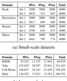
Book Set 1 2000 2000 2000 6000 Set 2 4824 513 663 6000 Electronics Set 1 2000 2000 2000 6000 Set 2 4817 694 489 6000 Beauty Set 1 2000 2000 2000 6000 Set 2 4709 616 675 6000 Music Set 1 2000 2000 2000 6000 Set 2 4441 785 774 6000

(a) Small-scale datasets

Domain #Pos #Neg #Neu Total

IMDB 55,242 11,735 17,942 84,919 Yelp 155,625 29,597 45,941 231,163 Cell Phone 148,657 24,343 21,439 194,439 Baby 126,525 17,012 17,255 160,792

(b) Large-scale datasets

Table 1: Summary of datasets.

4 Experiments

4.1 CNN Encoder Implementation

We have left the feature encoder G unspecified, for which, a few options can be considered. In our implementation, we adopt a one-layer CNN structure from previous works (Kim,2014;Yu and Jiang,2016), as it has been demonstrated to work well for sentiment classification tasks. Given a re-view documentx = (x1, x2, ..., xn)consisting of

nwords, we begin by associating each word with a continuous word embedding (Mikolov et al.,

2013)ex from an embedding matrixE 2 RV⇥d,

whereV is the vocabulary size anddis the embed-ding dimension. E is jointly updated with other network parameters during training. Given a win-dow of dense word embeddings ex1,ex2, ...,exl,

the convolution layer first concatenates these vec-tors to form a vectorxˆ of lengthld and then the output vector is computed by Equation (7):

Conv(ˆx) =f(W_·ˆx+b) (7)

✓g = {W, b} is the parameter set of the

en-coder G and is shared across all windows of the sequence. f is an element-wise non-linear activa-tion funcactiva-tion. The convoluactiva-tion operaactiva-tion can cap-ture local contextual dependencies of the input se-quence and the extracted feature vectors are sim-ilar to n-grams. After the convolution operation is applied to the whole sequence, we obtain a list of hidden vectorsH = (h1,h2, ...,hn). A

max-over-time pooling layer is applied to obtain the fi-nal vector representation⇠of the input document.

4.2 Datasets and Experimental Settings Existing benchmark datasets such as the Amazon benchmark (Blitzer et al.,2007) typically remove

reviews with neutral labels in both domains. This is problematic as the label information of the tar-get domain is not accessible in an unsupervised domain adaptation setting. Furthermore, remov-ing neutral instances may bias the dataset favor-ably for max-margin-based algorithms like ours, since the resulting dataset has all uncertain labels removed, leaving only high confidence examples. Therefore, we construct new datasets by ourselves. The results on the original Amazon benchmark is qualitatively similar, and we present them in Ap-pendixAfor completeness since most of previous works reported results on it.

Small-scale datasets: Our new dataset was de-rived from the large-scale Amazon datasets2

re-leased by McAuley et al. (2015). It contains four domains3_{: Book (BK), Electronics (E), Beauty}

(BT), and Music (M). Each domain contains two datasets. Set 1 contains 6000 instances with ex-actly balanced class labels, and set 2 contains 6000 instances that are randomly sampled from the large dataset, preserving the original label dis-tribution, which we believe better reflects the label distribution in real life. The examples in these two sets do not overlap. Detailed statistics of the gen-erated datasets are given in Table1a.

In all our experiments on the small-scale datasets, we use set 1 of the source domain as the only source with sentiment label information dur-ing traindur-ing, and we evaluate the trained model on set 1 of the target domain. Since we cannot con-trol the label distribution of unlabeled data during training, we consider two different settings:

Setting (1):Only set 1 of the target domain is used

as the unlabeled set. This tells us how the method performs in a condition when the target domain has a close-to-balanced label distribution. As we also evaluate on set 1 of the target domain, this is also considered as a transductive setting.

Setting (2): Set 2 from both the source and target

domains are used as unlabeled sets. Since set 2 is directly sampled from millions of reviews, it better reflects real-life sentiment distribution.

Large-scale datasets: We further conduct ex-periments on four much larger datasets: IMDB4

2_{http://jmcauley.ucsd.edu/data/amazon/}

3_{The original reviews were rated on a 5-point scale. We}

label them with rating<3,>3, and= 3as negative, posi-tive, and neutral respectively.

4_{IMDB is rated on a 10-point scale, and we label reviews}

(I), Yelp2014 (Y), Cell Phone (C), and Baby (B). IMDB and Yelp2014 were previously used in (Tang et al., 2015; Yang et al., 2017). Cell phone and Baby are from the large-scale Amazon dataset (McAuley et al., 2015;He and McAuley,

2016). Detailed statistics are summarized in Ta-ble1b. We keep all reviews in the original datasets and consider a transductive setting where all target examples are used for both training (without la-bel information) and evaluation. We perform sam-pling to balance the classes of labeled source data in each minibatchB(s)during training.

4.3 Selection of Development Set

Ideally, the development set should be drawn from the same distribution as the test set. However, un-der the unsupervised domain adaptation setting, we do not have any labeled target data at training phase which could be used as development set. In all of our experiments, for each pair of domains, we instead sample 1000 examples from the train-ing set of the source domain as development set. We train the network for a fixed number of epochs, and the model with the minimum classification er-ror on this development set is saved for evaluation. This approach works well on most of the problems since the target domain is supposed to behave like the source domain if the domain difference is ef-fectively reduced.

Another problem is how to select the values for hyper-parameters. If we tune 1 and 2 directly

on the development set from the source domain, most likely both of them will be set to 0, as un-labeled target data is not helpful for improving in-domain accuracy of the source in-domain. Other neu-ral network models also have the same problem for hyper-parameter tuning. Therefore, our strategy is to use the development set from the target domain to optimize 1 and 2 for one problem (e.g., we

only do this on E!BK), and fix their values on the other problems. This setting assumes that we have at least two labeled domains such that we can op-timize the hyper-parameters, and then we fix them for other new unlabeled domains to transfer to.

4.4 Training Details and Hyper-parameters We initialize word embeddings using the 300-dimension GloVe vectors supplied by Pennington et al., (2014), which were trained on 840 billion tokens from the Common Crawl. For each pair of domains, the vocabulary consists of the top 10000 most frequent words. For words in the vocabulary

but not present in the pre-trained embeddings, we randomly initialize them.

We set hyper-parameters of the CNN en-coder following previous works (Kim, 2014; Yu and Jiang, 2016) without specific tuning on our datasets. The window size is set to 3 and the size of the hidden layer is set to 300. The nonlinear activation function is Relu. For regularization, we also follow their settings and employ dropout with probability set to 0.5 on⇠ibefore feeding it to the

output layer F, and constrain the l2-norm of the

weight vector✓f, setting its max norm to 3.

On the small-scale datasets and the Aamzon benchmark, 1 and 2 are set to 200 and 1,

respectively, tuned on the development set of task E!BK under setting 1. On the large-scale

datasets, 1 and 2 are set to 500 and 0.2,

re-spectively, tuned on I!Y. We use a Gaussian curvew(t) = exp[ 5(1 _t t

max)

2_]

3 to ramp up

the weight of the bootstrapping loss⌦ from0 to 3, wheretmax denotes the maximum number of

training epochs. We train 30 epochs for all exper-iments. We set 3 to 3 and↵to 0.5 for all

experi-ments.

The batch size is set to 50 on the small-scale datasets and the Amazon benchmark. We increase the batch size to 250 on the large-scale datasets to reduce the number of iterations. RMSProp opti-mizer with learning rate set to 0.0005 is used for all experiments.

4.5 Models for Comparison

We compare with the following baselines:

(1) Naive: A non-domain-adaptive baseline with bag-of-words representations and SVM clas-sifier trained on the source domain.

(2)mSDA(Chen et al.,2012): This is the state-of-the-art method based on discrete input features. Top 1000 bag-of-words features are kept as pivot features. We set the number of stacked layers to 3 and the corruption probability to 0.5.

(3) NaiveNN: This is a non-domain-adaptive CNN trained on source domain, which is a variant of our model by setting 1, 2, and 3to zeros.

(4)AuxNN(Yu and Jiang,2016): This is a neu-ral model that exploits auxiliary tasks, which has achieved state-of-the-art results on cross-domain sentiment classification. The sentence encoder used in this model is the same as ours.

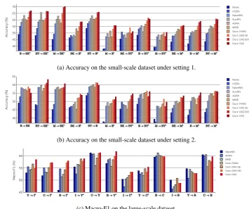
representa-40 45 50 55 60 65

70 Naive

mSDA NaiveNN AuxNN ADAN MMD Ours: FANN Ours: DAS-SE Ours: DAS-EM Ours: DAS

Accuracy (%)

(a) Accuracy on the small-scale dataset under setting 1.

40 45 50 55 60 65

Naive mSDA NaiveNN AuxNN ADAN MMD Ours: FANN Ours: DAS-SE Ours: DAS-EM Ours: DAS

Accuracy (%)

(b) Accuracy on the small-scale dataset under setting 2.

45 50 55 60

NaiveNN ADAN MMD Ours: FANN Ours: DAS-SE Ours: DAS-EM Ours: DAS

Ma

cro

-F

1

(%

)

(c) Macro-F1 on the large-scale dataset.

Figure 1: Performance comparison. Average results over 5 runs with random initializations are reported for each neural method. ⇤ _{indicates that the proposed method (either of DAS, DAS-EM, DAS-SE) is}

significantly better than other baselines (baseline 1-6) withp <0.05based on one-tailed unpaired t-test.

tion difference between domains. The original pa-per uses a simple feedforward network as encoder. For fair comparison, we replace it with our CNN-based encoder. We train 5 iterations on the dis-criminator per iteration on the encoder and senti-ment classifier as suggested in their paper.

(6)MMD: MMD has been widely used for min-imizing domain discrepancy on images. In those works (Tzeng et al.,2014;Long et al.,2017), vari-ants of deep CNNs are used for encoding images and the MMDs of multiple layers are jointly mini-mized. In NLP, adding more layers of CNNs may not be very helpful and thus those models from image-related tasks can not be directly applied to our problem. To compare with MMD-based method, we train a model that jointly minimize the classification lossLon the source domain and MMD between {⇠_i(s)|ns

i=1} and {⇠ (t)

i |ni=1t }. For

computing MMD, we use a Gaussian RBF which is a common choice for characteristic kernel.

In addition to the above baselines, we also show results of different variants of our model. DAS as shown in Algorithm1 denotes our full model. DAS-EM denotes the model with only entropy

minimization for semi-supervised learning (set

3 = 0). DAS-SEdenotes the model with only

self-ensemble bootstrapping for semi-supervised learning (set 2 = 0). FANN(feature-adaptation

neural network) denotes the model without semi-supervised learning performed (set both 2and 3

to zeros).

4.6 Main Results

Figure15_{shows the comparison of adaptation}

re-sults (see Appendix B for the exact numerical numbers). We report classification accuracy on the small-scale dataset. For the large-scale dataset, macro-F1 is instead used since the label distribu-tion in the test set is extremely unbalanced. Key observations are summarized as follows. (1) Both DAS-EM and DAS-SE perform better in most cases compared with ADAN, MDD, and FANN, in which only feature adaptation is performed. This demonstrates the effectiveness of the

pro-5_{We exclude results of Naive, mSDA and AuxNN on the}

0 0.1 0.2 0.3 0.4 0.5 0.6 0.7 0.8 0.9 1 55

60 65

DAS MMD ADAN

(a) Percentage of unlabeled target examples (BT->BK)

Accu

ra

cy

(%

)

0 0.1 0.2 0.3 0.4 0.5 0.6 0.7 0.8 0.9 1

45 50 55

DAS MMD ADAN

(b) Percentage of unlabeled target examples (M->E)

Accu

ra

cy

(%

)

0 0.1 0.2 0.3 0.4 0.5 0.6 0.7 0.8 0.9 1 50

55 60

DAS MMD ADAN

(c) Percentage of unlabeled target examples (E->BT)

Accu

ra

cy

(%

)

Figure 2: Accuracy vs. percentage of unlabeled target training examples.

0 50 100 150 200 250 300 350 400 450 500 60

65 70

DAS MMD ADAN NaiveNN

(a) # of labeled target examples (BT->BK)

Accu

ra

cy

(%

)

0 50 100 150 200 250 300 350 400 450 500 50

55 60

DAS MMD ADAN NaiveNN

(b) # of labeled target examples (M->E)

Accu

ra

cy

(%

)

0 50 100 150 200 250 300 350 400 450 500 55

60 65

DAS MMD ADAN NaiveNN

(c) # of labeled target examples (E->BT)

Accu

ra

cy

(%

)

Figure 3: Accuracy vs. number of labeled target training examples.

posed domain adaptive semi-supervised learning framework. EM is more effective than DAS-SE in most cases, and the full model DAS with both techniques jointly employed overall has the best performance. (2) When comparing the two settings on the small-scale dataset, all domain-adaptive methods6_{generally perform better under}

setting 1. In setting 1, the target examples are bal-anced in classes, which can provide more diverse opinion-related features. However, when consid-ering unsupervised domain adaptation, we should not presume the label distribution of the unlabeled data. Thus, it is necessary to conduct experiments using datasets that reflect real-life sentiment dis-tribution as what we did on setting2 and the large-scale dataset. Unfortunately, this is ignored by most of previous works. (3) Word-embeddings are very helpful, as we can see even NaiveNN can sub-stantially outperform mSDA on most tasks.

To see the effect of semi-supervised learning alone, we also conduct experiments by setting

1 = 0to eliminate the effect of feature

adapta-tion. Both entropy minimization and bootstrap-ping perform very badly in this setting. En-tropy minimization gives almost random predic-tions with accuracy below 0.4, and the results of bootstrapping are also much lower compared to NaiveNN. This suggests that the feature adap-tation component is essential. Without it, the learned target representations are less meaning-ful and discriminative. Applying semi-supervised

6_{Results of Naive and NaiveNN do not change under both}

settings as they are only trained on the source domain.

learning in this case is likely to worsen the results.

4.7 Further Analysis

In Figure2, we show the change of accuracy with respect to the percentage of unlabeled data used for training on three particular problems under set-ting 1. The value atx= 0denotes the accuracies of NaiveNN which does not utilize any target data. For DAS, we observe a nonlinear increasing trend where the accuracy quickly improves at the be-ginning, and then gradually stabilizes. For other methods, this trend is less obvious, and adding more unlabeled data sometimes even worsen the results. This finding again suggests that the pro-posed approach can better exploit the information from unlabeled data.

We also conduct experiments under a setting with a small number of labeled target examples available. Figure3shows the change of accuracy with respect to the number of labeled target exam-ples added for training. We can observe that DAS is still more effective under this setting, while the performance differences to other methods gradu-ally decrease with the increasing number of la-beled target examples.

4.8 CNN Filter Analysis

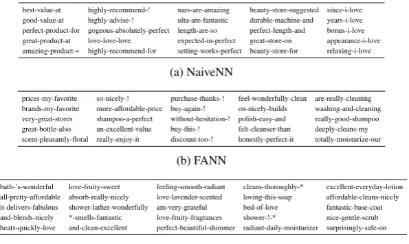
best-value-at highly-recommend-! nars-are-amazing beauty-store-suggested since-i-love

good-value-at highly-advise-! ulta-are-fantastic durable-machine-and years-i-love

perfect-product-for gogeous-absolutely-perfect length-are-so perfect-length-and bonus-i-love

great-product-at love-love-love expected-in-perfect great-store-on appearance-i-love

amazing-product-⇤ highly-recommend-for setting-works-perfect beauty-store-for relaxing-i-love

(a) NaiveNN

prices-my-favorite so-nicely-! purchase-thanks-! feel-wonderfully-clean are-really-cleaning

brands-my-favorite more-affordable-price buy-again-! on-nicely-builds washing-and-cleaning

very-great-stores shampoo-a-perfect without-hesitation-! polish-easy-and really-good-shampoo

great-bottle-also an-excellent-value buy-this-! felt-cleanser-than deeply-cleans-my

scent-pleasantly-floral really-enjoy-it discount-too-! honestly-perfect-it totally-moisturize-our

(b) FANN

bath-’s-wonderful love-fruity-sweet feeling-smooth-radiant cleans-thoroughly-* excellent-everyday-lotion

all-pretty-affordable absorb-really-nicely love-lavender-scented loving-this-soap affordable-cleans-nicely

it-delivers-fabulous shower-lather-wonderfully am-very-grateful bed-of-love fantastic-base-coat

and-blends-nicely *-smells-fantastic love-fruity-fragrances shower-!-* nice-gentle-scrub

heats-quickly-love and-clean-excellent perfect-beautiful-shimmer radiant-daily-moisturizer surprisingly-safe-on

(c) DAS

Table 2: Comparison of the top trigrams (each column) from the target domain (beauty) captured by the 5 most positive-sentiment-related CNN filters learned on E!BT.⇤denotes a padding.

of the output layer F. Higher weight indicates

stronger relatedness. 2) Recall that in our im-plementation, each CNN filter has a window size of 3 with Relu activation. We can thus represent each selected filter as a ranked list of trigrams with highest activation values.

We analyze the CNN filters learned by NaiveNN, FANN and DAS respectively on task E!BT under setting 1. We focus on E!BT for study because electronics and beauty are very dif-ferent domains and each of them has a diverse set of domain-specific sentiment expressions. For each method, we identify the top 10 most related filters for each sentiment label, and extract the top trigrams of each selected filter on both source and target domains. Since labeled source examples are used for training, we find the filters learned by the three methods capture similar expressions on the source domain, containing both domain-invariant and domain-specific trigrams. On the target do-main, DAS captures more target-specific expres-sions compared to the other two methods. Due to space limitation, we only present a small sub-set of positive-sentiment-related filters in Table2. The complete results are provided in AppendixC. From Table 2, we can observe that the filters learned by NaiveNN are almost unable to cap-ture target-specific sentiment expressions, while FANN is able to capture limited target-specific words such as “clean” and “scent”. The filters learned by DAS are more domain-adaptive, cap-turing diverse sentiment expressions in the target domain.

5 Conclusion

In this work, we propose DAS, a novel frame-work that jointly performs feature adaptation and semi-supervised learning. We have demonstrated through multiple experiments that DAS can better leverage unlabeled data, and achieve substantial improvements over baseline methods. We have also shown that feature adaptation is an essen-tial component, without which, semi-supervised learning is not able to function properly. The pro-posed framework could be potentially adapted to other domain adaptation tasks, which is the focus of our future studies.

References

John Blitzer, Mark Dredze, and Fernando Pereira. 2007. Biographies, Bollywood, boom-boxes and blenders: domain adaptation for sentiment classifi-cation. In Annual Meeting of the Association for Computational Linguistics.

Minmin Chen, Zhixiang Xu, Kilian Q. Weinberger, and Fei Sha. 2012. Marginalized denoising autoen-coders for domain adaptation. InThe 29th Interna-tional Conference on Machine Learning.

Xilun Chen, Yu Sun, Ben Athiwarakun, Claire Cardie, and Kilian Weinberger. 2017. Adversarial deep av-eraging networks for cross-lingual sentiment classi-fier. InArxiv e-prints arXiv:1606.01614.

Yaroslav Ganin and Victor Lempitsky. 2015. Unsuper-vised domain adaptation by backpropagation. In In-ternational Conference on Machine Learning.

Xavier Glorot, Antoine Bordes, and Yoshua Bengio. 2011. Domain adaptation for large-scale sentiment classification: a deep learning approach. InThe 28th International Conference on Machine Learning.

Yves Grandvalet and Yoshua Bengio. 2004. Semi-supervised learning by entropy minimization. In

Neural Information Processing Systems.

Arthur Gretton, Karsten M. Borgwardt, Malte J. Rasch, Bernhard Sch¨olkopf, and Alexander Smola. 2012. A kernel two-sample test. Journal of Machine Learn-ing Research, 13:723–773.

Ruining He and Julian McAuley. 2016. Ups and downs: modeling the visual evolution of fashion trends with one-class collaborative filtering. In

WWW.

Yulan He, Chenghua Lin, and Harith Alani. 2011. Automatically extracting polarity-bearing topics for cross-domain sentiment classification. InACL.

Jing Jiang and ChengXiang Zhai. 2007. Instance weighting for domain adaptation in NLP. InAnnual Meeting of the Association for Computational Lin-guistics.

Yoon Kim. 2014. Convolutional neural networks for sentence classification. InConference on Empirical Methods in Natural Language Processing.

Samuli Laine and Timo Aila. 2017. Temporal ensem-bling for semi-supervised learning. InInternational Conference on Learning Representation.

Zheng Li, Yun Zhang, Ying Wei, Yuxiang Wu, and Qiang Yang. 2017. End-to-end adversarial mem-ory network for cross-domain sentiment classifica-tion. InThe 26th International Joint Conference on Artificial Intelligence.

Mingsheng Long, Yue Cao, Jianmin Wang, and Michael I. Jordan. 2015. Learning transferable fea-tures with deep adaptation networks. In Interna-tional Conference on Machine Learning.

Mingsheng Long, Han Zhu, Jianmin Wang, and Michael I. Jordan. 2017. Deep transfer learning with joint adaptation networks. InInternational Confer-ence on Machine Learning.

Julian J. McAuley, Christopher Targett, Qinfeng Shi, and Anton van den Hengel. 2015. Image-based rec-ommendations on styles and substitutes. InThe 38th International ACM SIGIR Conference on Research and Development in Information Retrieval.

Tomas Mikolov, Ilya Sutskever, Kai Chen, Greg Cor-rado, and Jeffrey Dean. 2013. Distributed represen-tations of words and phrases and their composition-ality. InNeural Information Processing Systems.

Sinno Jialin Pan, Xiaochuan Ni, Jian-Tao Sun, Qiang Yang, and Zheng Chen. 2010. Cross-domain senti-ment classification via spectral feature alignsenti-ment. In

The 19th International World Wide Web Conference.

Jeffrey Pennington, Richard Socher, and Christopher D Manning. 2014. GloVe: Global vectors for word representation. In Conference on Empirical Meth-ods in Natural Language Processing.

Duyu Tang, Bing Qin, and Ting Liu. 2015. Learn-ing semantic representation of users and products for document level sentiment classification. InAnnual Meeting of the Association for Computational Lin-guistics.

Eric Tzeng, Judy Hoffman, Ning Zhang, Kate Saenko, and Trevor Darrell. 2014. Deep domain confusion: maximizing for domain invariance. InArxiv e-prints arXiv:1412.3474.

Dan Wu, Wee Sun Lee, Nan Ye, and Hai Leong Chieu. 2009. Domain adaptive bootstrapping for named en-tity recognition. InConference on Empirical Meth-ods in Natural Language Processing.

Fangzhao Wu and Yongfeng Huang. 2016. Sentiment domain adaptation with multiple sources. InAnnual Meeting of the Association for Computational Lin-guistics.

Wei Yang, Wei Lu, and Vincent W. Zheng. 2017. A simple regularization-based algorithm for learning cross-domain word embeddings. InConference on Empirical Methods in Natural Language Process-ing.

Yi Yang and Jacob Eisenstein. 2014. Fast easy unsu-pervised domain adaptation with marginalized struc-tured dropout. InAnnual Meeting of the Association for Computational Linguistics.

Jianfei Yu and Jing Jiang. 2016. Learning sentence em-beddings with auxiliary tasks for cross-domain sen-timent classification. In Conference on Empirical Methods in Natural Language Processing.

Guangyou Zhou, Tingting He, Wensheng Wu, and Xi-aohua Tony Hu. 2015. Linking heterogeneous input features with pivots for domain adaptation. InThe 24th International Joint Conference on Artificial In-telligence.

Guangyou Zhou, Zhiwen Xie, Jimmy Xiangji Huang, and Tingting He. 2016. Bi-transferring deep neural networks for domain adaptation. InAnnual Meeting of the Association for Computational Linguistics. Fuzhen Zhuang, Xiaohu Cheng, Ping Luo, Sinno Jialin