Incremental Skip-gram Model with Negative Sampling
Nobuhiro Kaji and Hayato Kobayashi Yahoo Japan Corporation
{nkaji,hakobaya}@yahoo-corp.jp
Abstract
This paper explores an incremental train-ing strategy for the skip-gram model with negative sampling (SGNS) from both em-pirical and theoretical perspectives. Ex-isting methods of neural word embed-dings, including SGNS, are multi-pass al-gorithms and thus cannot perform incre-mental model update. To address this problem, we present a simple incremen-tal extension of SGNS and provide a thorough theoretical analysis to demon-strate its validity. Empirical experiments demonstrated the correctness of the theo-retical analysis as well as the practical use-fulness of the incremental algorithm.
1 Introduction
Existing methods of neural word embeddings are typically designed to go through the entire train-ing data multiple times. For example, negative sampling (Mikolov et al., 2013b) needs to pre-compute the noise distribution from the entire training data before performing Stochastic Gradi-ent DescGradi-ent (SGD). It thus needs to go through the training data at least twice. Similarly, hierarchical soft-max (Mikolov et al., 2013b) has to determine the tree structure and GloVe (Pennington et al., 2014) has to count co-occurrence frequencies be-fore performing SGD.
The fact that those existing methods are multi-pass algorithms means that they cannot perform incremental model update when additional train-ing data is provided. Instead, they have to re-train the model on the old and new training data from scratch.
However, the re-training is obviously inefficient since it has to process the entire training data received thus far whenever new training data is
provided. This is especially problematic when the amount of the new training data is relatively smaller than the old one. One such situation is that the embedding model is updated on a small amount of training data that includes newly emerged words for instantly adding them to the vocabulary set. Another situation is that the word embeddings are learned from ever-evolving data such as news articles and microblogs (Peng et al., 2017) and the embedding model is periodically updated on newly generated data (e.g., once in a week or month).
This paper investigates an incremental training method of word embeddings with a focus on the skip-gram model with negative sampling (SGNS) (Mikolov et al., 2013b) for its popularity. We present a simple incremental extension of SGNS, referred to as incremental SGNS, and provide a thorough theoretical analysis to demonstrate its validity. Our analysis reveals that, under a mild assumption, the optimal solution of incremental SGNS agrees with the original SGNS when the training data size is infinitely large. See Section 4 for the formal and strict statement. Additionally, we present techniques for the efficient implemen-tation of incremental SGNS.
Three experiments were conducted to assess the correctness of the theoretical analysis as well as the practical usefulness of incremental SGNS. The first experiment empirically investigates the validity of the theoretical analysis result. The second experiment compares the word embed-dings learned by incremental SGNS and the orig-inal SGNS across five benchmark datasets, and demonstrates that those word embeddings are of comparable quality. The last experiment explores the training time of incremental SGNS, demon-strating that it is able to save much training time by avoiding expensive re-training when additional training data is provided.
2 SGNS Overview
As a preliminary, this section provides a brief overview of SGNS.
Given a word sequence, w1, w2, . . . , wn, for
training, the skip-gram model seeks to minimize the following objective to learn word embeddings:
LSG =−1n
n
∑
i=1 ∑
|j|≤c j̸=0
logp(wi+j |wi),
where wi is a target word and wi+j is a context
word within a window of size c. p(wi+j | wi)
represents the probability thatwi+jappears within
the neighbor ofwi, and is defined as
p(wi+j |wi) = ∑exp(twi·cwi+j) w∈Wexp(twi·cw)
, (1)
wheretwandcw arew’s embeddings when it
be-haves as a target and context, respectively.W rep-resents the vocabulary set.
Since it is too expensive to optimize the above objective, Mikolov et al. (2013b) proposed nega-tive sampling to speed up skip-gram training. This approximates Eq. (1) using sigmoid functions and krandomly-sampled words, called negative sam-ples. The resulting objective is given as
LSGNS=−n1
n
∑
i=1 ∑
|j|≤c j̸=0
ψ+
wi,wi+j+kEv∼q(v)[ψw−i,v],
whereψ+
w,v = logσ(tw·cv),ψ−w,v = logσ(−tw·
cv), andσ(x) is the sigmoid function. The
nega-tive samplev is drawn from a smoothed unigram probability distribution referred to asnoise distri-bution: q(v) ∝f(v)α, wheref(v)represents the
frequency of a wordvin the training data andαis a smoothing parameter (0< α≤1).
The objective is optimized by SGD. Given a target-context word pair (wi and wi+j) and k
negative samples (v1, v2, . . . , vk) drawn from the
noise distribution, the gradient of −ψ+
wi,wi+j − kEv∼q(v)[ψw−i,v] ≈ −ψ+wi,wi+j −
∑k
k′=1ψw−i,vk′ is computed. Then, the gradient descent is per-formed to updatetwi,cwi+j, andcv1, . . . ,cvk.
SGNS training needs to go over the entire train-ing data to pre-compute the noise distributionq(v)
before performing SGD. This makes it difficult to perform incremental model update when addi-tional training data is provided.
3 Incremental SGNS
This section explores incremental training of SGNS. The incremental training algorithm (Sec-tion 3.1), its efficient implementa(Sec-tion (Sec(Sec-tion 3.2), and the computational complexity (Section 3.3) are discussed in turn.
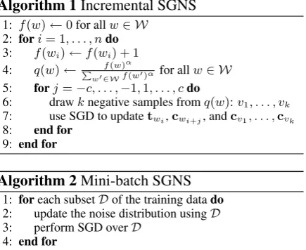
3.1 Algorithm
Algorithm 1 presents incremental SGNS, which goes through the training data in a single-pass to update word embeddings incrementally. Unlike the original SGNS, it does not pre-compute the noise distribution. Instead, it reads the training data word by word1 to incrementally update the word frequency distribution and the noise distribu-tion while performing SGD. Hereafter, the origi-nal SGNS (c.f., Section 2) is referred to asbatch SGNS to emphasize that the noise distribution is computed in a batch fashion.
The learning rate for SGD is adjusted by using AdaGrad (Duchi et al., 2011). Although the linear decay function has widely been used for training batch SGNS (Mikolov, 2013), adaptive methods such as AdaGrad are more suitable for the incre-mental training since the amount of training data is unknown in advance or can increase unboundedly. It is straightforward to extend the incremental SGNS to the mini-batch setting by reading a sub-set of the training data (or mini-batch), rather than a single word, at a time to update the noise distri-bution and perform SGD (Algorithm 2). Although this paper primarily focuses on the incremental SGNS, the mini-batch algorithm is also important in practical terms because it is easier to be multi-threaded.
Alternatives to Algorithms 2 might be possi-ble. Other possible approaches include computing the noise distribution separately on each subset of the training data, fixing the noise distribution after computing it from the first (possibly large) subset, and so on. We exclude such alternatives from our investigation because it is considered difficult to provide them with theoretical justification.
3.2 Efficient implementation
Although the incremental SGNS is conceptually simple, implementation issues are involved.
1In practice, Algorithm 1 buffers a sequence of words
Algorithm 1Incremental SGNS
1: f(w)←0for allw∈ W 2: fori= 1, . . . , ndo
3: f(wi)←f(wi) + 1 4: q(w)← f(w)α
∑
w′∈Wf(w′)αfor allw∈ W
5: forj=−c, . . . ,−1,1, . . . , cdo
6: drawknegative samples fromq(w):v1, . . . , vk 7: use SGD to updatetwi,cwi+j, andcv1, . . . ,cvk
8: end for
9: end for
Algorithm 2Mini-batch SGNS
1: foreach subsetDof the training datado
2: update the noise distribution usingD 3: perform SGD overD
4: end for
3.2.1 Dynamic vocabulary
One problem that arises when training incremen-tal SGNS is how to maintain the vocabulary set. Since new words emerge endlessly in the train-ing data, the vocabulary set can grow unboundedly and exhaust a memory.
We address this problem by dynamically chang-ing the vocabulary set. The Misra-Gries algorithm (Misra and Gries, 1982) is used to approximately keep track of top-m frequent words during train-ing, and those words are used as the dynamic vo-cabulary set. This method allows the maximum vocabulary size to be explicitly limited tom, while being able to dynamically change the vocabulary set.
3.2.2 Adaptive unigram table
Another problem is how to generate negative sam-ples efficiently. Since k negative samples per target-context pair have to be generated by the noise distribution, the sampling speed has a sig-nificant effect on the overall training efficiency.
[image:3.595.74.292.66.244.2]Let us first examine how negative samples are generated in batch SGNS. In a popular implemen-tation (Mikolov, 2013), a word array (referred to as a unigram table) is constructed such that the number of a wordwin it is proportional to q(w). See Table 1 for an example. Using the unigram table, negative samples can be efficiently gener-ated by sampling the table elements uniformly at random. It takes onlyO(1) time to generate one negative sample.
The above method assumes that the noise dis-tribution is fixed and thus cannot be used directly for the incremental training. One simple solution is to reconstruct the unigram table whenever new training data is provided. However, such a method
w a b c
q(w) 0.5 0.3 0.2 T = (a, a, a, a, a, b, b, b, c, c)
Table 1: Example noise distributionq(w) for the vocabulary setW ={a, b, c}(left) and the corre-sponding unigram tableTof size10(right).
Algorithm 3Adaptive unigram table.
1: f(w)←0for allw∈ W 2: z←0
3: fori= 1, . . . , ndo
4: f(wi)←f(wi) + 1
5: F ←f(wi)α−(f(wi)−1)α 6: z←z+F
7: if|T|< τthen
8: addFcopies ofwitoT 9: else
10: forj= 1, . . . , τdo
11: T[j]←wiwith probabilityFz
12: end for
13: end if
14: end for
is not effective for the incremental SGNS, because the unigram table reconstruction requiresO(|W|)
time.2
We propose a reservoir-based algorithm for ef-ficiently updating the unigram table (Vitter, 1985; Efraimidis, 2015) (Algorithm 3). The algorithm incrementally update the unigram table T while limiting its maximum size toτ. In case|T|< τ, it can be easily confirmed that the number of a word winT isf(w)α(∝q(w)). In case|T|=τ, since
z = ∑w∈Wf(w)α is equal to the normalization
factor of the noise distribution, it can be proven by induction that, for allj,T[j]is a wordwwith probability q(w). See (Vitter, 1985; Efraimidis, 2015) for reference.
Note on implementation In line 8,F copies of
wiare added to T. When F is not an integer, the
copies are generated so that their expected number becomesF. Specifically,⌈F⌉copies are added to T with probabilityF − ⌊F⌋, and⌊F⌋copies are added otherwise.
The loop from line 10 to 12 becomes expen-sive if implemented straightforwardly because the maximum table size τ is typically set large (e.g.,
τ = 108 inword2vec(Mikolov, 2013)). For
ac-celeration, instead of checking all elements in the unigram table, randomly chosen τF
z elements are
substituted withwi. Note that τFz is the expected
2This overhead is amortized in mini-batch SGNS if the
[image:3.595.307.528.161.308.2]number of table elements to be substituted in the original algorithm. This approximation achieves great speed-up because we usually haveF ≪ z. In fact, it can be proven that it takes O(1) time whenα= 1.0. See Appendix3A for more discus-sions.
3.3 Computational complexity
Both incremental and batch SGNS have the same space complexity, which is independent of the training data sizen. Both require O(|W|) space to store the word embeddings and the word fre-quency counts, andO(|T|)space to store the uni-gram table.
The two algorithms also have the same time complexity. Both requireO(n)training time when the training data size is n. Although incremen-tal SGNS requires extra time for updating the dynamic vocabulary and adaptive unigram table, these costs are practically negligible, as will be demonstrated in Section 5.3.
4 Theoretical Analysis
Although the extension from batch to incremental SGNS is simple and intuitive, it is not readily clear whether incremental SGNS can learn word em-beddings as well as the batch counterpart. To an-swer this question, in this section we examine in-cremental SGNS from a theoretical point of view. The analysis begins by examining the difference between the objectives optimized by batch and in-cremental SGNS (Section 4.1). Then, probabilis-tic properties of their difference are investigated to demonstrate the relationship between batch and incremental SGNS (Sections 4.2 and 4.3). We shortly touch the mini-batch SGNS at the end of this section (Section 4.4).
4.1 Objective difference
As discussed in Section 2, batch SGNS optimizes the following objective:
LB(θ)=−n1
n
∑
i=1 ∑
|j|≤c j̸=0
ψ+
wi,wi+j+kEv∼qn(v)[ψw−i,v],
whereθ= (t1,t2, . . . ,t|W|,c1,c2, . . . ,c|W|)
col-lectively represents the model parameters4 (i.e., word embeddings) andqn(v)represents the noise
3The appendices are in the supplementary material. 4We treat words as integers and thusW={1,2, . . .|W|}.
distribution. Note that the noise distribution is rep-resented in a different notation than Section 2 to make its dependence on the whole training data explicit. The functionqi(v)is defined asqi(v) =
fi(v)α
∑
v′∈Wfi(v′)α, where fi(v) represents the word frequency in the firstiwords of the training data.
In contrast, incremental SGNS computes the gradient of−ψ+
wi,wi+j −kEv∼qi(v)[ψw−i,v]at each step to perform gradient descent. Note that the noise distribution does not depend onnbut rather oni. Because it can be seen as a sample approxi-mation of the gradient of
LI(θ) =−n1
n
∑
i=1 ∑
|j|≤c j̸=0
ψw+i,wi+j+kEv∼qi(v)[ψ−wi,v],
incremental SGNS can be interpreted as optimiz-ingLI(θ)with SGD.
Since the expectation terms in the objec-tives can be rewritten as Ev∼qi(v)[ψ−
wi,v] = ∑
v∈Wqi(v)ψ−wi,v, the difference between the two objectives can be given as
∆L(θ) =LB(θ)− LI(θ)
= n1 ∑n
i=1 ∑
|j|≤c j̸=0
k∑
v∈W
(qi(v)−qn(v))ψ−wi,v
= 2ckn
n
∑
i=1 ∑
v∈W
(qi(v)−qn(v))ψw−i,v
= 2ckn ∑
w,v∈W
n
∑
i=1
δwi,w(qi(v)−qn(v))ψw,v−
whereδw,v =δ(w=v)is the delta function.
4.2 Unsmoothed case
Let us begin by examining the objective difference
∆L(θ)in the unsmoothed case,α= 1.0.
We below introduce some definitions and nota-tions as the preparation of the analysis.
Definition 1. LetXi,w be a random variable that
representsδwi,w. It takes1when thei-th word in the training data isw∈ Wand0otherwise.
Remind that we assume that the words in the training data are generated from a stationary dis-tribution. This assumption means that the expec-tation and (co)variance ofXi,w do not depend on
the index i. Hereafter, they are respectively de-noted asE[Xi,w] =µwandV[Xi,w,Xj,v] =ρw,v.
Definition 2. LetYi,w be a random variable that
represents qi(w) when α = 1.0. It is given as
Yi,w = 1i ∑ii′=1Xi′,w.
4.2.1 Convergence of the first and second
order moments of∆L(θ)
It can be shown that the first order moment of
∆L(θ)has an analytical form.
Theorem 1. The first order moment of∆L(θ)is
given as
E[∆L(θ)] = 2ck(Hn−1)
n
∑
w,v∈W
ρw,vψ−w,v,
whereHnis then-th harmonic number.
Sketch of proof. Notice that E[∆L(θ)] can be written as
2ck n
∑
w,v∈W
n
∑
i=1 (
E[Xi,wYi,v]−E[Xi,wYn,v])ψw,v− .
Because we have, for anyiandjsuch thati≤j,
E[Xi,wYj,v] =
j
∑
j′=1
E[Xi,wXjj′,v] =µwµv+ρw,vj ,
plugging this into E[∆L(θ)]proves the theorem. See Appendix B.1 for the complete proof.
Theorem 1 readily gives the convergence prop-erty of the first order moment of∆L(θ):
Theorem 2. The first-order moment of∆L(θ)
de-creases in the order ofO(log(nn)):
E[∆L(θ)] =O
(
log(n)
n )
,
and thus converges to zero in the limit of infinity:
lim
n→∞E[∆L(θ)] = 0.
Proof. We have Hn= O(log(n)) from the
up-per integral bound, and thus Theorem 1 gives the proof.
A similar result to Theorem 2 can be obtained for the second order moment of∆L(θ)as well.
Theorem 3. The second-order moment of∆L(θ)
decreases in the order ofO(log(nn)):
E[∆L(θ)2] =O(log(n)
n )
,
and thus converges to zero in the limit of infinity:
lim
n→∞E[∆L(θ)
2] = 0.
Proof. Omitted. See Appendix B.2. 4.2.2 Main result
The above theorems reveal the relationship be-tween the optimal solutions of the two objectives, as stated in the next lemma.
Lemma 4. Let θ∗ and θˆ be the optimal
solu-tions of LB(θ) and LI(θ), respectively: θ∗ =
arg minθLB(θ)andθˆ= arg minθLI(θ). Then, lim
n→∞E[LB(ˆθ)− LB(θ∗)] = 0, (2)
lim
n→∞V[LB(ˆθ)− LB(θ∗)] = 0. (3)
Proof. The proof is made by the squeeze theorem. Let l = LB(ˆθ)− LB(θ∗). The optimality of θ∗ gives0≤l. Also, the optimality ofθˆgives
l=LB(ˆθ)− LI(θ∗) +LI(θ∗)− LB(θ∗) ≤ LB(ˆθ)− LI(ˆθ) +LI(θ∗)− LB(θ∗) = ∆L(ˆθ)−∆L(θ∗).
We thus have0 ≤ E[l] ≤ E[∆L(ˆθ)−∆L(θ∗)].
Since Theorem 2 implies that the right hand side converges to zero whenn→ ∞, the squeeze the-orem gives Eq. (2). Next, we have
V[l] =E[l2]−E[l]2 ≤E[l2]
≤E[(∆L(ˆθ)−∆L(θ∗))2]
≤E[(∆L(ˆθ)−∆L(θ∗))2]
+E[(∆L(ˆθ)+∆L(θ∗))2]
We are now ready to provide the main result of the analysis. The next theorem shows the conver-gence ofLB(ˆθ).
Theorem 5. LB(ˆθ) converges in probability to
LB(θ∗):
∀ϵ >0, lim
n→∞Pr
[
|LB(ˆθ)− LB(θ∗)| ≥ϵ
]
= 0.
Sketch of proof. Let again l = LB(ˆθ) − LB(θ∗). Chebyshev’s inequality gives, for anyϵ1 >0,
lim
n→∞ V[l]
ϵ2
1 ≥nlim→∞Pr [
|l−E[l]| ≥ϵ1 ]
.
Remember that Eq. (2) means that for anyϵ2 >0, there existsn′ such that ifn′≤nthen|E[l]|< ϵ
2. Therefore, we have
lim
n→∞ V[l]
ϵ2
1 ≥nlim→∞Pr [
|l| ≥ϵ1+ϵ2 ]
≥0.
The arbitrary property of ϵ1 and ϵ2 allows ϵ1 + ϵ2 to be rewritten asϵ. Also, Eq. (3) implies that
limn→∞ Vϵ[2l]
1 = 0. This completes the proof. See
Appendix B.3 for the detailed proof.
Informally, this theorem can be interpreted as sug-gesting that the optimal solutions of batch and in-cremental SGNS agree whennis infinitely large.
4.3 Smoothed case
We next examine the smoothed case (0< α <1). In this case, the noise distribution can be repre-sented by using the ones in the unsmoothed case:
qi(w) = fi(w) α
∑
w′∈Wfi(w′)α =
(fi(w)
Fi )α ∑
w′∈W(fi(Fwi′))α
whereFi =∑w′∈Wfi(w′)and fiF(wi)corresponds
to the unsmoothed noise distribution.
Definition 3. LetZi,w be a random variable that
represents qi(w) in the smoothed case. Then, it
can be written by usingYi,w:
Zi,w=gw(Yi,1,Yi,2, . . . ,Yi,|W|)
wheregw(x1, x2, . . . , x|W|) = x
α w
∑
w′∈Wxαw′. Because Zi,w is no longer a linear
combina-tion of Xi,w, it becomes difficult to derive
simi-lar proofs to the unsmoothed case. To address this
difficulty, Zi,w is approximated by the first-order
Taylor expansion around
E[(Yi,1,Yi,2, . . . ,Yi,|W|)] = (µ1, µ2, . . . , µ|W|).
The first-order Taylor approximation gives
Zi,w≈gw(µ) +
∑
v∈W
Mw,v(Yi,v−gv(µ))
where µ = (µ1, µ2, . . . , µ|W|) and Mw,v = ∂gw(x)
∂xv |x=µ. Consequently, it can be shown that the first and second order moments of∆L(θ)have the order of O(log(nn)) in the smoothed case as well. See Appendix C for the details.
4.4 Mini-batch SGNS
The same analysis result can also be obtained for the mini-batch SGNS. We can prove Theorems 2 and 3 in the mini-batch case as well (see Ap-pendix D for the proof). The other part of the anal-ysis remains the same.
5 Experiments
Three experiments were conducted to investigate the correctness of the theoretical analysis (Sec-tion 5.1) and the practical usefulness of incremen-tal SGNS (Sections 5.2 and 5.3). Details of the experimental settings that do not fit into the paper are presented in Appendix E.
5.1 Validation of theorems
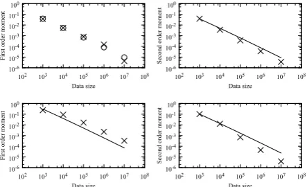
An empirical experiment was conducted to vali-date the result of the theoretical analysis. Since it is difficult to assess the main result in Section 4.2.2 directly, the theorems in Sections 4.2.1, from which the main result is readily derived, were in-vestigated. Specifically, the first and second order moments of∆L(θ)were computed on datasets of increasing sizes to empirically investigate the con-vergence property.
Datasets of various sizes were constructed from the English Gigaword corpus (Napoles et al., 2012). The datasets made up of n words were constructed by randomly sampling sentences from the Gigaword corpus. The value ofnwas varied over {103,104,105,106,107}. 10,000 different datasets were created for each size nto compute the first and second order moments.
10-6 10-5 10-4 10-3 10-2 10-1 100
102 103 104 105 106 107 108
First order moment
Data size
10-6
10-5
10-4
10-3
10-2
10-1
100
102 103 104 105 106 107 108
Second order moment
Data size
10-6 10-5 10-4 10-3 10-2 10-1 100
102 103 104 105 106 107 108
First order moment
Data size
10-6
10-5
10-4
10-3
10-2
10-1
100
102 103 104 105 106 107 108
Second order moment
[image:7.595.74.296.65.200.2]Data size
Figure 1: Log-log plots of the first and second order moments of ∆L(θ) on the different sized datasets whenα= 1.0(top left and top right) and α= 0.75(bottom left and bottom right).
and circles represent the empirical values and the-oretical values obtained by Theorem 1, respec-tively. Figure 1 (top right) similarly illustrates the second order moments of ∆L(θ). Since Theo-rem 3 suggests that the second order moment de-creases in the order ofO(log(nn)), the graph y ∝
log(x)
x is also shown. The graph was fitted to the
empirical data by minimizing the squared error. The top left figure demonstrates that the empiri-cal values of the first order moments fit the theoret-ical result very well, providing a strong empirtheoret-ical evidence for the correctness of Theorem 1. In ad-dition, the two figures show that the first and sec-ond order moments decrease almost in the order ofO(log(nn)), converging to zero as the data size increases. This result validates Theorems 2 and 3. Figures 1 (bottom left) and (bottom right) show similar results when α = 0.75. Since we do not have theoretical estimates of the first order mo-ment when α ̸= 1.0, the graphs y ∝ log(nn) are shown in both figures. From these, we can again observe that the first and second order moments decrease almost in the order of O(log(nn)). This indicates the validity of the investigation in Sec-tion 4.3. The relatively larger deviaSec-tions from the graphs y ∝ log(nn), compared with the top right figure, are considered to be attributed to the first-order Taylor approximation.
5.2 Quality of word embeddings
The next experiment investigates the quality of the word embeddings learned by incremental SGNS through comparison with the batch counterparts.
The Gigaword corpus was used for the training.
For the comparison, both our own implementation of batch SGNS as well as WORD2VEC (Mikolov
et al., 2013c) were used (denoted as batch and w2v). The training configurations of the three methods were set the same as much as possible, although it is impossible to do so perfectly. For ex-ample, incremental SGNS (denoted as incremen-tal) utilized the dynamic vocabulary (c.f., Section 3.2.1) and thus we set the maximum vocabulary sizemto control the vocabulary size. On the other hand, we set a frequency threshold to determine the vocabulary size ofw2v. We setm = 240k for
incremental, while setting the frequency
thresh-old to100forw2v. This yields vocabulary sets of comparable sizes:220,389and246,134.
The learned word embeddings were assessed on five benchmark datasets commonly used in the literature (Levy et al., 2015): WordSim353 (Agirre et al., 2009), MEN (Bruni et al., 2013), SimLex-999 (Hill et al., 2015), the MSR analogy dataset (Mikolov et al., 2013c), the Google anal-ogy dataset (Mikolov et al., 2013a). The former three are for a semantic similarity task, and the remaining two are for a word analogy task. As evaluation measures, Spearman’sρand prediction accuracy were used in the two tasks, respectively.
Figures 2 (a) and (b) represent the results on the similarity datasets and the analogy datasets. We see that the three methods (incremental, batch, and w2v) perform equally well on all of the datasets. This indicates that incremental SGNS can learn as good word embeddings as the batch counterparts, while being able to perform incre-mental model update. Althoughincremental per-forms slightly better than the batch methods in some datasets, the difference seems to be a prod-uct of chance.
The figures also show the results of incremen-tal SGNS when the maximum vocabulary sizem was reduced to150k and100k (incremental-150k
andincremental-100k). The resulting vocabulary
0.2 0.4 0.6 0.8 1
WordSim353 MEN SimLex999
Spearman's
ρ
incremental incremental-150k incremental-100k batch w2v
0.2 0.4 0.6 0.8 1
Google MSR
Accuracy
incremental incremental-150k incremental-100k batch w2v
0 5 10 15
1 2 3 4 5
Update time (10
3 sec.)
Size of new training data (×106)
incremental batch w2v
(a) (b) (c)
Figure 2: (a): Spearman’sρon the word similarity datasets. (b): Accuracy on the analogy datasets. (c): Update time when new training data is provided.
5.3 Update time
The last experiment investigates how much time incremental SGNS can save by avoiding re-training when updating the word embeddings.
In this experiment, incremental was first trained on the initial training data of size5n
1 and then updated on the new training data of sizen2to measure the update time. For comparison,batch andw2vwere re-trained on the combination of the initial and new training data. We fixedn1 = 107 and variedn2over{1×106,2×106, . . . ,5×106}. The experiment was conducted on Intel⃝R Xeon⃝R
2GHz CPU. The update time was averaged over five trials.
Figure 2 (c) compares the update time of the three methods across various values ofn2. We see
thatincrementalsignificantly reduces the update
time. It achieves10and7.3times speed-up com-pared withbatchandw2v(whenn2 = 106). This represents the advantage of the incremental algo-rithm, as well as the time efficiency of the dynamic vocabulary and adaptive unigram table. We note
thatbatchis slower thanw2vbecause it uses
Ada-Grad, which maintains different learning rates for different dimensions of the parameter, whilew2v uses the same learning rate for all dimensions.
6 Related Work
Word representations based on distributional se-mantics have been common (Turney and Pantel, 2010; Baroni and Lenci, 2010). The distributional methods typically begin by constructing a word-context matrix and then applying dimension re-duction techniques such as SVD to obtain high-quality word meaning representations. Although some studies investigated incremental updating of the word-context matrix (Yin et al., 2015; Goyal
5The number of sentences here.
and Daume III, 2011), they did not explore the re-duced representations. On the other hand, neural word embeddings have recently gained much pop-ularity as an alternative. However, most previous studies have not explored incremental strategies (Mikolov et al., 2013a,b; Pennington et al., 2014). Peng et al. (2017) proposed an incremental learning method of hierarchical soft-max. Be-cause hierarchical soft-max and negative sampling have different advantages (Peng et al., 2017), the incremental SGNS and their method are com-plementary to each other. Also, their updating method needs to scan not only new but also old training data, and thus is not an incremental algo-rithm in a strict sense. As a consequence, it poten-tially incurs the same time complexity as the re-training. Another consequence is that their method has to retain the old training data and thus wastes space, while incremental SGNS can discard old training examples after processing them.
Very recently, May et al. (2017) also proposed an incremental algorithm for SGNS. However, their work differs from ours in that their algorithm is not designed to use smoothed noise distribution (i.e., the smoothing parameterαis assumed fixed as α = 1.0 in their method), which is a key to learn high-quality word embeddings. Another dif-ference is that they did not provide theoretical jus-tification for their algorithm.
There are publicly available implementations for training SGNS, one of the most popular being
WORD2VEC (Mikolov, 2013). However, it does
not support an incremental training method. GEN -SIM( ˇReh˚uˇrek and Sojka, 2010) also offers SGNS
training. Although GENSIMallows the
incremen-tal updating of SGNS models, it is done in an ad-hoc manner. In GENSIM, the vocabulary set as
[image:8.595.79.517.65.169.2]they do not provide any theoretical accounts for the validity of their training method. Finally, we want to note that most of the existing implemen-tations can be easily extended to support the in-cremental (or mini-batch) SGNS by simply keep updating the noise distribution.
7 Conclusion and Future Work
This paper proposed incremental SGNS and pro-vided thorough theoretical analysis to demonstrate its validity. We also conducted experiments to em-pirically demonstrate its effectiveness. Although the incremental model update is often required in practical machine learning applications, only a lit-tle attention has been paid to learning word em-beddings incrementally. We consider that incre-mental SGNS successfully addresses this situation and serves as an useful tool for practitioners.
The success of this work suggests several re-search directions to be explored in the future. One possibility is to explore extending other embed-ding methods such as GloVe (Pennington et al., 2014) to incremental algorithms. Such studies would further extend the potential of word embed-ding methods.
References
Eneko Agirre, Enrique Alfonseca, Keith Hall, Jana Kravalova, Marius Pasca, and Aitor Soroa. 2009. A study on similarity and relatedness using distribu-tional and wordnet-based approaches. In
Proceed-ings of NAACL, pages 19–27.
Marco Baroni and Alessandro Lenci. 2010. Dis-tributional memory: A general framework for corpus-based semantics. Computatoinal Linguis-tics, 36:673–721.
E. Bruni, N. K. Tran, and M. Baroni. 2013. Multi-modal distributional semantics. Journal of Artificial Intelligence Research, 49:1–49.
John Duchi, Elad Hazan, and Yoram Singer. 2011. Adaptive subgradient methods for online learning and stochastic optimization. Journal of Machine
Learning Research, 12:2121–2159.
Pavlos S. Efraimidis. 2015. Weighted random sam-pling over data streams. ArXiv:1012.0256.
Amit Goyal and Hal Daume III. 2011. Approximate scalable bounded space sketch for large data nlp. In
Proceedings of EMNLP, pages 250–261.
Felix Hill, Roi Reichart, and Anna Korhonen. 2015. Simlex-999: Evaluating semantic models with (gen-uine) similarity estimation. Computational Linguis-tics, 41:665–695.
Omer Levy, Yoav Goldberg, and Ido Dagan. 2015. Im-proving distributional similarity with lessons learned from word embeddings. Transactions of the Associ-ation for ComputAssoci-ational Linguistics, 3:211–225. Chandler May, Kevin Duh, Benjamin Van Durme,
and Ashwin Lall. 2017. Streaming word em-beddings with the space-saving algorithm. ArXiv:1704.07463.
Tomas Mikolov. 2013. word2vec. https://code.google.com/archive/p/word2vec. Tomas Mikolov, Kai Chen, Greg Corrado, and Jeffrey
Dean. 2013a. Efficient estimation of word represen-tations in vector space. InWorkshop at ICLR. Tomas Mikolov, Ilya Sutskever, Kai Chen, Greg S
Cor-rado, and Jeff Dean. 2013b. Distributed representa-tions of words and phrases and their compositional-ity. InAdvances in NIPS, pages 3111–3119. Tomas Mikolov, Wen-Tau Yih, and Geoffrey Zweig.
2013c. Linguistic regularities in continuous space word representations. In Proceedings of NAACL, pages 746–751.
Jayadev Misra and David Gries. 1982. Finding re-peated elements. Science of Computer Program-ming, 2(2):143–152.
Courtney Napoles, Matthew Gormley, and Ben-jamin Van Durme. 2012. Annotated english giga-word ldc2012t21.
Hao Peng, Jianxin Li, Yangqiu Song, and Yaopeng Liu. 2017. Incrementally learning the hierarchical soft-max function for neural language models. In
Pro-ceedings of AAAI, pages 3267–3273.
Jeffrey Pennington, Richard Socher, and Christopher Manning. 2014. Glove: Global vectors for word representation. In Proceedings of EMNLP, pages 1532–1543.
Radim ˇReh˚uˇrek and Petr Sojka. 2010. Software frame-work for topic modelling with large corpora. In Pro-ceedings of the LREC 2010 Workshop on New
Chal-lenges for NLP Frameworks, pages 45–50.
Peter D. Turney and Patrick Pantel. 2010. From fre-quency to meaning: Vector space models of se-mantics. Journal of Artificial Intelligence Research, 37:141–188.
Jeffrey S. Vitter. 1985. Random sampling with a reser-voir. ACM Transactions on Mathematical Software, 11:37–57.