Proceedings of the 2016 Conference on Empirical Methods in Natural Language Processing, pages 469–478,
The Structured Weighted Violations Perceptron Algorithm
Rotem Dror and Roi Reichart
Faculty of Industrial Engineering and Management, Technion, IIT {rtmdrr@campus|roiri@ie}.technion.ac.il
Abstract
We present theStructured Weighted Violations Perceptron (SWVP) algorithm, a new struc-tured prediction algorithm that generalizes the Collins Structured Perceptron (CSP, (Collins, 2002)). Unlike CSP, the update rule of SWVP explicitly exploits the internal structure of the predicted labels. We prove the convergence of SWVP for linearly separable training sets, provide mistake and generalization bounds, and show that in the general case these bounds are tighter than those of the CSP special case. In synthetic data experiments with data drawn from an HMM, various variants of SWVP substantially outperform its CSP special case. SWVP also provides encouraging initial de-pendency parsing results.
1 Introduction
The structured perceptron ((Collins, 2002), hence-forth denoted CSP) is a prominent training algo-rithm for structured prediction models in NLP, due to its effective parameter estimation and simple im-plementation. It has been utilized in numerous NLP applications including word segmentation and POS tagging (Zhang and Clark, 2008), dependency pars-ing (Koo and Collins, 2010; Goldberg and Elhadad, 2010; Martins et al., 2013), semantic parsing (Zettle-moyer and Collins, 2007) and information extrac-tion (Hoffmann et al., 2011; Reichart and Barzilay, 2012), if to name just a few.
Like some training algorithms in structured pre-diction (e.g. structured SVM (Taskar et al., 2004; Tsochantaridis et al., 2005), MIRA (Crammer and Singer, 2003) and LaSo (Daum´e III and Marcu,
2005)), CSP considers in its update rule the differ-ence betweencompletepredicted and gold standard labels (Sec. 2). Unlike others (e.g. factored MIRA (McDonald et al., 2005b; McDonald et al., 2005a) and dual-loss based methods (Meshi et al., 2010)) it does not exploit the structure of the predicted label. This may result in valuable information being lost.
Consider, for example, the gold and predicted de-pendency trees of Figure 1. The substantial differ-ence between the trees may be mostly due to the dif-ference in roots (are andworse, respectively). Pa-rameter update w.r.t this mistake may thus be more useful than an update w.r.t the complete trees.
In this work we present a new perceptron algo-rithm with an update rule that exploits the struc-ture of a predicted label when it differs from the gold label (Section 3). Our algorithm is calledThe Structured Weighted Violations Perceptron (SWVP) as its update rule is based on a weighted sum of up-dates w.r.t violating assignmentsand non-violating assignments: assignments to the input example, de-rived from the predicted label, that score higher (for violations) and lower (for non-violations) than the gold standard label according to the current model.
Our concept ofviolating assignment is based on Huang et al. (2012) that presented a variant of the CSP algorithm where the argmax inference problem is replaced with a violation finding function. Their update rule, however, is identical to that of the CSP algorithm. Importantly, although CSP and the above variant do not exploit the internal structure of the predicted label, they are special cases of SWVP.
In Section 4 we prove that for a linearly separable training set, SWVP converges to a linear separator of
the data under certain conditions on the parameters of the algorithm, that are respected by the CSP spe-cial case. We further prove mistake and generaliza-tion bounds for SWVP, and show that in the general case the SWVP bounds are tighter than the CSP’s.
In Section 5 we show that SWVP allows ag-gressiveupdates, that exploit only violating assign-ments derived from the predicted label, and more balanced updates, that exploit both violating and non-violating assignments. In experiments with syn-thetic data generated by an HMM, we demonstrate that various SWVP variants substantially outper-form CSP training. We also provide initial encour-aging dependency parsing results, indicating the po-tential of SWVP for real world NLP applications.
2 The Collins Structured Perceptron In structured prediction the task is to find a mapping
f : X → Y, where y ∈ Y is a structured object
rather than a scalar, and a feature mappingφ(x, y) :
X × Y(x) → Rdis given. In this work we denote
Y(x) = {y0|y0 ∈DYLx}, whereLx, a scalar, is the
size of the allowed output sequence for an input x
andDY is the domain ofy0ifor everyi∈ {1, . . . Lx}.
1 Our results, however, hold for the general case of an output space with variable size vectors as well.
The CSP algorithm (Algorithm 1) aims to learn a parameter (or weight) vector w ∈ Rd, that
sepa-rates the training data, i.e. for each training example
(x, y)it holds that:y= arg maxy0∈Y(x)w·φ(x, y0).
To find such a vector the algorithm iterates over the training set examples and solves the above in-ference (argmax) problem. If the inferred label
y∗ differs from the gold label y the update w =
w+ ∆φ(x, y, y∗)is performed. For linearly
separa-ble training data (see definition 4), CSP is proved to converge to a vectorwseparating the training data.
Collins and Roark (2004) and Huang et al. (2012) expanded the CSP algorithm by proposing various alternatives to the argmaxinferenceproblem which is often intractable in structured prediction problems (e.g. in high-order graph-based dependency parsing (McDonald and Pereira, 2006)). The basic idea is re-placing the argmax problem with the search for a vi-olation: an output label that the model scores higher
1In the general caseL
xis a set of output sizes, which may be finite or infinite (as in constituency parsing (Collins, 1997)).
Algorithm 1The Structured Perceptron (CSP)
Input:dataD={xi, yi}n
i=1, feature mappingφ
Output:parameter vectorw∈Rd
Define:∆φ(x, y, z),φ(x, y)−φ(x, z)
1: Initializew= 0. 2: repeat
3: foreach(xi, yi)∈Ddo 4: y∗= arg max
y0∈Y(xi)w·
φ(xi, y0)
5: ify∗6=yithen
6: w=w+ ∆φ(xi, yi, y∗) 7: end if
8: end for
9: untilConvergence
than the gold standard label. The update rule in these CSP variants is, however, identical to the CSP’s. We, in contrast, propose a novel update rule that exploits the internal structure of the model’s prediction re-gardless of the way this prediction is generated.
3 The Structured Weighted Violations Perceptron (SWVP)
SWVP exploits the internal structure of a predicted label y∗ 6= y for a training example (x, y) ∈ D,
by updating the weight vector with respect to sub-structures ofy∗. We start by presenting the
funda-mental concepts at the basis of our algorithm. 3.1 Basic Concepts
Sub-structure Sets We start with two fundamen-tal definitions: (1)An individualsub-structureof a structured object (or label)y∈DYLx, denoted with
J, is defined to be a subset of indexes J ⊆ [Lx];2
and(2)Aset of substructuresfor a training example
(x, y), denoted withJJx, is defined asJJx⊆2[Lx].
Mixed Assignment We next define the concept of amixed assignment:
Definition 1. For a training pair(x, y) and a
pre-dicted label y∗ ∈ Y(x), y∗ 6= y, amixed
assign-ment (M A)vector denoted asmJ(y∗, y)is defined
with respect toJ ∈JJxas follows:
mJk(y∗, y) =
(
yk∗ k∈J
yk else
That is, a mixed assignment is a new label, de-rived from the predicted labely∗, that is identical to y∗ in all indexes inJ and toy otherwise. For
sim-plicity we denotemJ(y∗, y) = mJ when the
refer-encey∗ andylabels are clear from the context.
Consider, for example, the trees of Figure 1, as-suming that the top tree is y, the middle tree isy∗
andJ = [2,5].3 In themJ(y∗, y)(bottom) tree the
heads of all the words are identical to those of the top tree, except for the heads ofmistakesand ofthen. Violation The next central concept is that of a vi-olation, originally presented by Huang et al. (2012): Definition 2. A triple (x, y, y∗) is said to be a vio-lationwith respect to a training example(x, y)and a parameter vectorwif fory∗ ∈ Y(x)it holds that y∗6=yandw·∆φ(x, y, y∗)≤0.
The SWVP algorithm distinguishes between
M As that are violations, and ones that are not. For
a triplet(x, y, y∗)and a set of substructuresJJx ⊆
2[Lx]we provide the following notations:
I(y∗, y, JJx)v ={J∈JJx|mJ 6=y,w·∆φ(x, y, mJ)≤0}
I(y∗, y, JJx)nv={J∈JJx|mJ 6=y,w·∆φ(x, y, mJ)>0}
This notation divides the set of substructures into two subsets, one consisting of the substructures that yield violating MAs and one consisting of the substructures that yield non-violating MAs. Here again when the reference label y∗ and the set
JJx are known we denote: I(y∗, y, JJx)v = Iv,
I(y∗, y, JJx)nv=InvandI =Iv∪Inv.
Weighted Violations The key idea of SWVP is the exploitation of the internal structure of the pre-dicted label in the update rule. For this aim at each iteration we define the set of substructures,JJx, and
then, for eachJ ∈JJx, update the parameter vector,
w, with respect to the mixed assignments,M AJ’s.
This is a more flexible setup compared to CSP, as we can update with respect to the predicted output (if it is a violation, as is promised if inference is per-formed via argmax), if we wish to do so, as well as with respect to other mixed assignments.
Naturally, not all mixed assignments are equally important for the update rule. Hence, we weigh the different updates using a weight vectorγ. This
pa-per therefore extends the observation of Huang et al. (2012) that perceptron parameter update can be per-formed w.r.t violations (Section 2), by showing that wcan actually be updated w.r.t linear combinations of mixed assignments, under certain conditions on the selected weights.
3We index the dependency tree words from 1 onwards.
Some mistakes are worse than others.
Some mistakes are worse than others.
[image:3.612.364.493.59.130.2]Some mistakes are worse than others.
Figure 1:Example parse trees: gold tree (y, top), predicted tree (y∗, middle) with arcs differing from the gold’s marked with a dashed line, andmJ(y∗, y)forJ= [2,5](bottom tree).
3.2 Algorithm
With these definitions we can present the SWVP al-gorithm (Alal-gorithm 2). SWVP is in fact a family of algorithms differing with respect to two decisions that can be made at each pass over each training ex-ample(x, y): the choice of the setJJx and the
im-plementation of the SETGAMMAfunction.
SWVP is very similar to CSP except for in the update rule. Like in CSP, the algorithm iterates over the training data examples and for each example it first predicts a label according to the current param-eter vectorw(inference is discussed in Section 4.2, property 2). The main difference from CSP is in the update rule (lines 6-12). Here, for each substructure in the substructure set,J ∈JJx, the algorithm
gen-erates a mixed assignmentmJ (lines 7-9). Then,w
is updated with a weighted sum of the mixed assign-ments (line 11), unlike in CSP where the update is held w.r.t the predicted assignment only.
The γ(mJ) weights assigned to each of the ∆φ(x, y, mJ)updates are defined by a SETGAMMA
function (line 10). Intuitively, a γ(mJ) weight
should be higher the more the mixed assignment is assumed to convey useful information that can guide the update ofwin the right direction. In Sec-tion 4 we detail the condiSec-tions on SETGAMMA
un-der which SWVP converges, and in Section 5 we describe various SETGAMMAimplementations.
Going back to the example of Figure 1, one would assume (Sec. 1) that the head word prediction for worseis pivotal to the substantial difference between the two top trees (UAS of 0.2). CSP does not directly exploit this observation as it only updates its param-eter vector with respect to the differences between complete assignments:w=w+ ∆φ(x, y, z).
assignment for each of the erroneous arcs where all other words are assigned their correct arc (according to the gold tree) except for that specific arc which is kept as in the bottom tree. Then, higher weights can be assigned to errors that seem more central than others. We elaborate on this in the next two sections.
Algorithm 2The Structured Weighted Violations Perceptron
Input:dataD={xi, yi}n
i=1, feature mappingφ
Output:parameter vectorw∈Rd
Define:∆φ(x, y, z),φ(x, y)−φ(x, z)
1: Initializew= 0. 2: repeat
3: foreach(xi, yi)∈Ddo 4: y∗= arg max
y0∈Y(xi)w·
φ(xi, y0)
5: ify∗6=yithen 6: Define:JJxi⊆2[Lxi] 7: forJ∈JJxido 8: Define:mJs.t.mJ
k= (
yk∗ k∈J yi
k else 9: end for
10: γ=SETGAMMA()
11: w=w+ P
J∈Iv∪Invγ(m
J)∆φ(xi, yi, mJ)
12: end if
13: end for
14: untilConvergence
4 Theory
We start this section with the convergence conditions on theγvector which weighs the mixed assignment
updates in the SWVP update rule (line 11). Then, using these conditions, we describe the relation be-tween the SWVP and the CSP algorithms. After that, we prove the convergence of SWVP and anal-yse the derived properties of the algorithm.
γ Selection Conditions Our main observation in
this section is that SWVP converges under two con-ditions: (a)the training setDis linearly separable;
and (b) for any parameter vector w achievable by the algorithm, there exists(x, y) ∈ DwithJJx ⊆
2[Lx], such that for the predicted output y∗ 6= y,
SETGAMMAreturns aγ weight vector that respects
theγ selection conditions defined as follows:
Definition 3. The γ selection conditions for the
SWVP algorithm are (I =Iv∪Inv):
(1)X
J∈I
γ(mJ) = 1. γ(mJ)≥0, ∀J∈I.
(2) w·X J∈I
γ(mJ)∆φ(xi, yi, mJ)≤0.
With this definition we are ready to prove the fol-lowing property.
SWVP Generalizes the CSP Algorithm We now show that the CSP algorithm is a special case of SWVP. CSP can be derived from SWVP when tak-ing: JJx = {[Lx]}, and γ(m[Lx]) = 1 for every
(x, y) ∈ D. With these parameters, theγ selection conditions hold for everywand y∗. Condition (1)
holds trivially as there is only oneγcoefficient and it
is equal to 1. Condition (2) holds asy∗=m[Lx]and
henceI ={[Lx]}andw· P J∈I
∆φ(x, y, mJ)≤0.
4.1 Convergence for Linearly Separable Data Here we give the theorem regarding the convergence of the SWVP in the separable case. We first define: Definition 4. A data setD={xi, yi}ni=1islinearly
separable with marginδ > 0 if there exists some vectoruwithkuk2= 1such that for alli:
u·∆φ(xi, yi, z)≥δ,∀z∈ Y(xi).
Definition 5. The radius of a data set D =
{xi, yi}n
i=1is the minimal scalarRs.t for alli:
k∆φ(xi, yi, z)k ≤R,∀z∈ Y(xi). We next extend these definitions:
Definition 6. Given a data setD={xi, yi}n i=1and
a set JJ = {JJxi ⊆ 2[Lxi]|(xi, yi) ∈ D}, D is linearly separable w.r.t JJ, with margin δJJ > 0
if there exists a vector u with kuk2 = 1 such
that: u·∆φ(xi, yi, mJ(z, yi))≥ δJJ for alli, z ∈
Y(xi), J ∈JJ xi.
Definition 7.Themixed assignment radius w.r.tJJ
of a data setD= {xi, yi}n
i=1is a constantRJJ s.t
for alliit holds that:
k∆φ(xi, yi, mJ(z, yi))k ≤RJJ,∀z∈ Y(xi), J∈JJxi. With these definitions we can make the following observation (proof in A):
Observation 1. For linearly separable data Dand
a setJJ, every unit vectoruthat separates the data
with marginδ, also separates the data with respect to
mixed assignments withJJ, with marginδJJ ≥ δ.
Likewise, it holds thatRJJ ≤R.
We can now state our convergence theorem. While the proof of this theorem resembles that of the CSP (Collins, 2002), unlike the CSP proof the SWVP proof relies on theγselection conditions
Theorem 1. For any dataset D, linearly separable with respect toJJwith marginδJJ >0, the SWVP
algorithm terminates aftert ≤ ((RδJJJJ))22 steps, where
RJJ is the mixed assignment radius of D w.r.t.JJ.
Proof. Let wt be the weight vector before the tth
update, thusw1 = 0. Suppose thetthupdate occurs
on example (x, y), i.e. for the predicted outputy∗
it holds thaty∗ 6= y. We will boundkwt+1k2 from
both sides.
First, it follows from the update rule of the algorithm that: wt+1 = wt+ P
J∈Iv∪Inv
γ(mJ)∆φ(x, y, mJ).
For simplicity, in this proof we will use the notation
Iv ∪Inv =I. Hence, multiplying each side of the
equation byuyields: u·wt+1= u
·wt+u
·X
J∈I
γ(mJ)∆φ(x, y, mJ)
= u·wt+X J∈I
γ(mJ)u·∆φ(x, y, mJ)
≥ u·wt+X J∈I
γ(mJ)δJJ (margin property)
≥ u·wt+δJJ ≥. . .≥tδJJ.
The last inequality holds becausePJ∈Iγ(mJ) = 1. From this we get thatkwt+1k2 ≥(δJJ)2t2 since
kuk=1. Second,
kwt+1 k2=
kwt+X J∈I
γ(mJ)∆φ(x, y, mJ)k2
= kwt
k2+ kX
J∈I
γ(mJ)∆Φ(x, y, mJ)k2
+ 2wt
·X
J∈I
γ(mJ)∆Φ(x, y, mJ).
Fromγselection condition (2) we get that:
kwt+1k2≤ kwtk2+kX J∈I
γ(mJ)∆Φ(x, y, mJ)k2
≤ kwtk2+X J∈I
γ(mJ)k∆Φ(x, y, mJ)k2
≤ kwt
k2+ (RJJ)2. (radius property) The inequality one before the last results from the Jensen inequalitywhich holds due to(a)γselection
condition (1); and(b)the squared norm function be-ing convex. From this we finally get:
kwt+1k2≤ kwtk2+ (RJJ)2≤. . .≤t(RJJ)2. Combining the two steps we get:
(δJJ)2t2≤ kwt+1 k2
≤t(RJJ)2.
From this it is easy to derive the upper bound in the theorem: t≤ (RJJ)2
(δJJ)2 .
4.2 Convergence Properties
We next point on three properties of the SWVP al-gorithm, derived from its convergence proof:
Property 1 (tighter iterations bound) The con-vergence proof of CSP (Collins, 2002) is given for a vectoruthat linearly separates the data, with mar-ginδand for a data radiusR. Following observation
1, it holds that in our case,ualso linearly separates the data with respect to mixed assignments with a setJJ and with marginδJJ ≥δ. Together with the
definition ofRJJ ≤ R we get that: (RJJ)2
(δJJ)2 ≤ R 2
δ2.
This means that the bound on the number of updates made by SWVP is tighter than the bound of CSP.
Property 2 (inference)From theγselection
con-ditions it holds that any label from which at least one violating MA can be derived throughJJxis suitable
for an update. This is because in such a case we can choose, for example, a SETGAMMA function that
assigns the weight of 1 to that MA, and the weight of 0 to all other MAs.
Algorithm 2 employs theargmaxinference
func-tion, following the basic reasoning that it is a good choice to base the parameter update on. Importantly, if the inference function is argmax and the algorithm performs an update (y∗6=y), this means thaty∗, the
output of the argmax function, is a violating MA by definition. However, it is obvious that solving the in-ference problem and the optimalγassignment prob-lems jointly may result in more informed parameter (w) updates. We leave a deeper investigation of this issue to future research.
Property 3 (dynamic updates) The γ
selec-tion condiselec-tions paragraph states two condiselec-tions ((a) and (b)) under which the convergence proof holds. While it is trivial for SETGAMMA to generate a γ
vector that respects condition (a), if there is a pa-rameter vector w’ achievable by the algorithm for which SETGAMMAcannot generateγ that respects
condition (b), SWVP gets stuck when reachingw’. This problem can be solved with dynamic up-dates. A deep look into the convergence proof re-veals that the set JJx and the SETGAMMA
back off to the CSP setup of JJx = {[Lx]}, and
∀(x, y) ∈D :γ(m[Lx]) = 1, update its parameters
and continue with its originalJJ and SETGAMMA
when this option becomes feasible. If this does not happen, the algorithm can continue till convergence with the CSP setup.
4.3 Mistake and Generalization Bounds
The following bounds are proved: the number of updates in the separable case (see Theorem 1); the number of mistakes in the non-separable case (see Appendix B); and the probability to misclassify an unseen example (see supplementary material). It can be shown that in the general case these bounds are tighter than those of the CSP special case. We next discuss variants of SWVP.
5 Passive Aggressive SWVP
Here we present types of update rules that can be implemented within SWVP. Such rule types are de-fined by: (a) the selection ofγ, which should respect
theγ selection conditions(see Definition 3) and (b) the selection ofJJ = {JJx ⊆ 2[Lx]|(x, y) ∈ D},
the substructure sets for the training examples.
γSelection A first approach we consider is the
ag-gressive approach4 where only mixed assignments that are violations {mJ : J ∈ Iv} are exploited (i.e. for all J ∈ Inv, γ(mJ) = 0). Note, that in
this case condition (2) of theγ selection conditions
trivially holds as:w· P
J∈Iv
γ(mJ)∆φ(x, y, mJ)≤0.
The only remaining requirement is that condition (1) also holds, i.e. thatPJ∈Ivγ(mJ) = 1.
The opposite, passive approach, exploits only non-violating MA’s {mJ : J ∈ Inv}.
How-ever, such γ assignments do not respect γ
selection condition (2), as they yield: w ·
P
J∈Invγ(mJ)∆φ(x, y, mJ) ≤ 0 which holds if
and only if for everyJ ∈ Inv,γ(mJ) = 0 that in
turn contradicts condition (1).
Finally, we can take abalanced approachwhich gives a positiveγ coefficient for at least one
violat-ing MA and at least one positive γ coefficient for a non-violating MA. This approach is allowed by SWVP as long as bothγ selection conditions hold.
4We borrow the termpassive-aggressivefrom (Crammer et al., 2006), despite the substantial difference between the works.
We implemented two weighting methods, both based on the concept of margin:
(1) Weighted Margin (WM): γ(mJ) = |w·∆φ(x,y,mJ)|β
P
J0∈JJx|w·∆φ(x,y,m J0)|β
(2) Weighted Margin Rank (WMR):
γ(mJ) = |JJx|−r |JJx|
β
. where r is the
rank of |w · ∆φ(x, y, mJ(y∗, y))| among the
|w·∆φ(x, y, mJ0(y∗, y))|values forJ0 ∈JJx.
Both schemes were implemented twice, within a balanced approach (denoted as B) and an aggressive approach (denoted as A).5 The aggressive schemes respect bothγ selection conditions. The balanced
schemes, however, respect the first condition but not necessarily the second. Since all models that employ the balanced weighting schemes converged after at most 10 iterations, we did not impose this condition (which we could do by, e.g., excluding terms forJ ∈
Invtill condition (2) holds).
JJ Selection Another choice that strongly affects
the updates made by SWVP is that ofJJ. A choice ofJJx = 2[Lx],for every(x, y) ∈ Dresults in an
update rule which considers all possible mixing as-signments derived from the predicted label y∗ and the gold labely. Such an update rule, however,
re-quires computing a sum over an exponential number of terms (2Lx) and is therefore highly inefficient.
Among the wide range of alternative approaches, in this paper we exploitsingle differencemixed as-signments. In this approach we define: JJ =
{JJx = {{1},{2}, . . .{Lx}}|(x, y) ∈ D}. For a
training pair (x, y) ∈ D, a predicted label y∗ and J ={j} ∈JJx, we will have:
mJk(y∗, y) =
(
yk k6=j
yk∗ k=j
Under this approach for the pair(x, y) ∈Donly Lx terms are summed in the SWVP update rule.
We leave a further investigation ofJJselection
ap-proaches to future research.
6 Experiments
Synthetic Data We experiment with syn-thetic data generated by a linear-chain, first-5For the aggressive approach the equations for schemes (1) and (2) are changed such that JJx is replaced with
order Hidden Markov Model (HMM, (Ra-biner and Juang, 1986)). Our learning al-gorithm is a liner-chain conditional random field (CRF, (Lafferty et al., 2001)): P(y|x) =
1
Z(x)
Q
i=1:Lxexp(w ·φ(yi−1, yi, x)) (where Z(x)
is a normalization factor) with binary indicator fea-tures{xi, yi, yi−1,(xi, yi),(yi, yi−1),(xi, yi, yi−1)}
for the triplet(yi, yi−1, x).
A dataset is generated by iteratively samplingK
items, each is sampled as follows. We first sam-ple a hidden state, y1, from a uniform prior
distri-bution. Then, iteratively, for i = 1,2, . . . , Lx we
sample an observed state from the emission prob-ability and (for i < Lx) a hidden state from the
transition probability. We experimented in 3 setups. In each setup we generated 10 datasets that were subsequently divided to a 7000 items training set, a 2000 items development set and a 1000 items test set. In all datasets, for each item, we set Lx = 8.
We experiment in three conditions: (1) simple(++), learnable(+++), (2) simple(++), learnable(++) and (3) simple(+), learnable(+).6
For each dataset (3 setups, 10 datasets per setup) we train variants of the SWVP algorithm differing in theγ selection strategy (WM or WMR, Section 5),
being aggressive (A) or passive (B), and in theirβ
parameter (β = {0.5,1, . . . ,5}). Training is done on the training subset and the best performing vari-ant on the development subset is applied to the test subset. For CSP no development set is employed as there is no hyper-parameter to tune. We report averaged accuracy (fraction of observed states for which the model successfully predicts the hidden state value) across the test sets, together with the standard deviation.
Dependency Parsing We also report initial de-pendency parsing results. We implemented our algo-rithms within the TurboParser (Martins et al., 2013).
6Denoting D
x = [Cx], Dy = [Cy], and a permuta-tion of a vector vwith perm(v), the parameters of the dif-ferent setups are: (1) simple(++), learnable(+++): Cx =
5, Cy = 3, P(y0|y) = perm(0.7,0.2,0.1), P(x|y) =
perm(0.75,0.1,0.05,0.05,0.05). (2) simple(++), learn-able(++): Cx = 5,Cy = 3,P(y0|y) = perm(0.5,0.3,0.2),
P(x|y) = perm(0.6,0.15,0.1,0.1,0.05). (3) sim-ple(+), learnable(+): Cx = 20 , Cy = 7 ,
P(y0|y) = perm(0.7,0.2,0.1,0, . . . ,0)), P(x|y) =
perm(0.4,0.2,0.1,0.1,0.1,0, . . . ,0).
That is, every other aspect of the parser: feature set, probabilistic pruning algorithm, inference algo-rithm etc., is kept fixed but training is performed with SWVP. We compare our results to the parser performance with CSP training (which comes with the standard implementation of the parser).
We experiment with the datasets of the CoNLL 2007 shared task on multilingual dependency pars-ing (Nilsson et al., 2007), for a total of 9 languages. We followed the standard train/test split of these dataset. For SWVP, we randomly sampled 1000 sen-tences from each training set to serve as develop-ment sets and tuned the parameters as in the syn-thetic data experiments. CSP is trained on the train-ing set and applied to the test set without any devel-opment set involved. We report the Unlabeled At-tachment Score (UAS) for each language and model.
7 Results
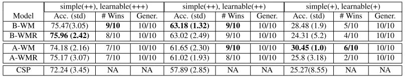
Synthetic Data Table 1 presents our results. In all three setups an SWVP algorithm is superior. Av-eraged accuracy differences between the best per-forming algorithms and CSP are: 3.72 (B-WMR, (simple(++), learnable(+++))), 5.29 (B-WM, ple(++), learnable(++))) and 5.18 (A-WM, (sim-ple(+), learnable(+))). In all setups SWVP outper-forms CSP in terms of averaged performance (ex-cept from B-WMR for (simple(+), learnable(+))). Moreover, the weighted models are more stable than CSP, as indicated by the lower standard deviation of their accuracy scores. Finally, for the more sim-ple and learnable datasets the SWVP models outper-form CSP in the majority of cases (7-10/10).
We measure generalization from development to test data in two ways. First, for each SWVP algo-rithm we count the number of times its β
parame-ter results in an algorithm that outperforms the CSP on the development set but not on the test set (not shown in the table). Of the 120 comparisons re-ported in the table (4 SWVP models, 3 setups, 10 comparisons per model/setup combination) this hap-pened once (A-MV, (simple(++), learnable(+++)).
Second, we count the number of times the best de-velopment set value of theβhyper-parameter is also the best value on the test set, or the test set accu-racy with the best development setβis at most 0.5%
Gener-simple(++), learnable(+++) simple(++), learnable(++) simple(+), learnable(+) Model Acc. (std) # Wins Gener. Acc. (std) # Wins Gener. Acc. (std) # Wins Gener. B-WM 75.47(3.05) 9/10 10/10 63.18 (1.32) 9/10 10/10 28.48 (1.9) 5/10 10/10 B-WMR 75.96 (2.42) 8/10 10/10 63.02 (2.49) 9/10 10/10 24.31 (5.2) 4/10 10/10 A-WM 74.18 (2.16) 7/10 10/10 61.65 (2.30) 9/10 10/10 30.45 (1.0) 6/10 10/10 A-WMR 75.17 (3.07) 7/10 10/10 61.02 (1.93) 8/10 10/10 25.8 (3.18) 2/10 10/10
[image:8.612.104.509.56.133.2]CSP 72.24 (3.45) NA NA 57.89 (2.85) NA NA 25.27(8.55) NA NA
Table 1: Overall Synthetic Data Results. A-andB-denote an aggressive and a balanced approaches, respectively. Acc. (std) is the average and the standard deviation of the accuracy across 10 test sets. # Wins is the number of test sets on which the SWVP algorithm outperforms CSP. Gener. is the number of times the bestβhyper-parameter value on the development set is also the best value on the test set, or the test set accuracy with the best development setβis at most 0.5% lower than that with the best test setβ.
First Order Second Order
Language CSP B-WM Top B-WM Test B-WM CSP B-WM Top B-WM Test B-WM
English 86.34 86.4 86.7 86.7 88.02 87.82 87.82 87.92
Chinese 84.60 84.5 85.04 85.05 86.82 86.69 86.83 87.02
Arabic 79.09 79.17 79.21 79.21 76.07 75.94 76.09 76.09
Greek 80.41 80.20 80.28 80.28 80.31 80.40 80.40 80.61
Italian 84.63 84.64 84.74 84.70 84.03 84.08 84.15 84.28
Turkish 83.05 82.89 82.89 82.89 83.02 83.04 83.04 83.31
Basque 79.47 79.54 79.54 79.54 80.52 80.57 80.63 80.64
Catalan 88.51 88.46 88.50 88.5 88.71 88.81 88.81 88.82
Hungarian 80.17 80.07 80.07 80.21 80.61 80.45 80.45 80.55
Average 83.69 83.65 83.77 83.79 83.12 83.08 83.13 83.35
Table 2:First and second order dependency parsing UAS results for CSP trained models, as well as for models trained with SWVP with a balancedγselection (B) and with a weighted margin (WM) strategy. For explanation of the B-WM, Top B-WM, and Test B-WM see text. For each language and parsing order we highlight the best result in bold font, but this do not include results from Test B-WM as it is provided only as an upper bound on the performance of SWVP.
alizationcolumn of the table shows that this has not happened in all of the 120 runs of SWVP.
Dependency Parsing Results are given in Table 2. For the SWVP trained models we report three numbers: (a) B-WM is the standard setup where the
βhyper parameter is tuned on the development data;
(b) For Top B-WM we first selected the models with a UAS score within 0.1% of the best development data result, and of these we report the UAS of the model that performs best on the test set; and (c) Test B-WM reports results whenβis tuned on the test set.
This measure provides an upper bound on SWVP with our simplisticJJ(Section 5).
Our results indicate the potential of SWVP. De-spite our simpleJJset, Top B-WM and Test B-WM
improve over CSP in 5/9 and 6/9 cases in first order parsing, respectively, and in 7/9 cases in second or-der parsing. In the latter case, Test B-WM improves the UAS over CSP in 0.22% on average across lan-guages. Unfortunately, SWVP still does not gener-alize well from train to test data as indicated, e.g., by the modest improvements B-WM achieves over CSP in only 5 of 9 languages in second order parsing.
8 Conclusions
We presented the Structured Weighted Violations Perceptron (SWVP) algorithm, a generalization of the Structured Perceptron (CSP) algorithm that ex-plicitly exploits the internal structure of the pre-dicted label in its update rule. We proved the conver-gence of the algorithm for linearly separable training sets under certain conditions on its parameters, and provided generalization and mistake bounds.
In experiments we explored only very simple con-figurations of the SWVP parameters - γ and JJ.
Nevertheless, several of our SWVP variants out-performed the CSP special case in synthetic data experiments. In dependency parsing experiments, SWVP demonstrated some improvements over CSP, but these do not generalize well. While we find these results somewhat encouraging, they emphasize the need to explore the much more flexible γ and JJ
A Proof Observation 1.
Proof. For every training example (x, y) ∈ D, it
holds that: ∪z∈Y(x)mJ(z, y) ⊆ Y(x). As u
sepa-rates the data with marginδ, it holds that:
u·∆φ(x, y, mJ(z, y))≥δJJx, ∀z∈ Y(x), J ∈JJ
x.
u·∆φ(x, y, z)≥δ, ∀z∈ Y(x).
Therefore also δJJx ≥ δ. As the last
inequal-ity holds for every(x, y) ∈ Dwe get that δJJ = min(x,y)∈DδJJx ≥δ.
From the same considerations it holds that RJJ ≤
R. This is because RJJ is the radius of a
sub-set of the datasub-set with radius R (proper subset if
∃(x, y) ∈ D,[Lx] ∈/ JJx, non-proper subset
oth-erwise).
B Mistake Bound - Non Separable Case Here we provide a mistake bound for the algorithm in the non-separable case. We start with the follow-ing definition and observation:
Definition 8. Given an example(xi, yi) ∈D, for a
u, δpair define:
ri=u·φ(xi, yi)− max
z∈Y(xi)u·φ(x
i, z)
i= max{0, δ−ri}
riJJ =u·φ(xi, yi)−
max
z∈Y(xi),J∈JJ xi
u·φ(xi, mJ(z, yi))
Finally define:Du,δ = s
n P i=1
2
i
Observation 2. For alli:ri ≤riJJ.
Observation 2 easily follows from Definition 8. Following this observation we denote: rdif f =
mini{riJJ −ri} ≥0and present the next theorem:
Theorem 2. For any training sequenceD, for the
first pass over the training set of the CSP and the SWVP algorithms respectively, it holds that:
#mistakes−CSP ≤ min
u:kuk=1,δ>0
(R+Du,δ)2
δ2 .
#mistakes−SW V P ≤ min
u:kuk=1,δ>0
(RJJ+Du,δ)2
(δ+rdif f)2 .
As RJJ ≤ R (Observation 1) and rdif f ≥ 0,
we get a tighter bound for SWVP. The proof for #mistakes-CSP is given at (Collins, 2002). The proof for #mistakes-SWVP is given below.
Proof. We transform the representation φ(x, y) ∈
Rdinto a new representationψ(x, y)∈Rd+nas
fol-lows: for i = 1, ..., d : ψi(x, y) = φi(x, y), for
j = 1, ..., n : ψd+j(x, y) = ∆if(x, y) = (xj, yj)
and0otherwise, where∆>0is a parameter.
Given a u, δ pair definev ∈ Rd+n as follows: for
i= 1, ..., d:vi =ui, forj = 1, ..., n:vd+j = ∆j.
Under these definitions we have:
v·ψ(xi, yi)−v·ψ(xi, z)≥δ, ∀i, z∈ Y(xi).
For everyi, z∈ Y(xi), J ∈JJ xi :
v·ψ(xi, yi)−v·ψ(xi, mJ(z, yi))≥δ+rdif f.
kψ(xi, yi)−ψ(xi, mJ(z, yi))k2 ≤(RJJ)2+ ∆2.
Last, we have,
kvk2=kuk2+
n X
i=1 2i
∆2 = 1 + Du2,δ
∆2 .
We get that the vector kvvk linearly separates the data with respect to single decision assignments with margin r δ
1+D
2 U,δ ∆2
. Likewise, kvvk linearly separates
the data with respect to mixed assignments withJJ,
with margin δ+rdif f r
1+D∆2u,δ
. Notice that the first pass
of SWVP with representation Ψ is identical to the
first pass with representationΦbecause the
param-eter weight for the additional features affects only a single example of the training data and do not affect the classification of test examples. By theorem 1 this means that thefirstpass of SWVP with representa-tionΨmakes at most (((Rδ+JJr)dif f2+∆)22)· 1 +
D2
u,δ
∆2
. We minimize this w.r.t ∆, which gives: ∆ =
p
RJJD
u,δ, and obtain the result guaranteed in the
theorem.
Acknowledgments
References
Michael Collins and Brian Roark. 2004. Incremental parsing with the perceptron algorithm. In Proc. of ACL.
Michael Collins. 1997. Three generative, lexicalised models for statistical parsing. InProc. of ACL, pages 16–23.
Michael Collins. 2002. Discriminative training methods for hidden markov models: Theory and experiments with perceptron algorithms. InProc. of EMNLP, pages 1–8.
Koby Crammer and Yoram Singer. 2003. Ultraconser-vative online algorithms for multiclass problems. The Journal of Machine Learning Research, 3:951–991. Koby Crammer, Ofer Dekel, Joseph Keshet, Shai
Shalev-Shwartz, and Yoram Singer. 2006. Online passive-aggressive algorithms. The Journal of Machine Learn-ing Research, 7:551–585.
Hal Daum´e III and Daniel Marcu. 2005. Learning as search optimization: Approximate large margin meth-ods for structured prediction. InProc. of ICML, pages 169–176.
Yoav Freund and Robert E Schapire. 1999. Large margin classification using the perceptron algorithm. Machine learning, 37(3):277–296.
Yoav Goldberg and Michael Elhadad. 2010. An effi-cient algorithm for easy-first non-directional depen-dency parsing. InProc. of NAACL-HLT 2010, pages 742–750.
Raphael Hoffmann, Congle Zhang, Xiao Ling, Luke Zettlemoyer, and Daniel S Weld. 2011. Knowledge-based weak supervision for information extraction of overlapping relations. InProc. of ACL.
Liang Huang, Suphan Fayong, and Yang Guo. 2012. Structured perceptron with inexact search. In Proc. of NAACL-HLT, pages 142–151.
Terry Koo and Michael Collins. 2010. Efficient third-order dependency parsers. InProc. of ACL, pages 1– 11.
John Lafferty, Andrew McCallum, and Fernando CN Pereira. 2001. Conditional random fields: Probabilis-tic models for segmenting and labeling sequence data. InProc. of ICML.
Andr´e FT Martins, Miguel Almeida, and Noah A Smith. 2013. Turning on the turbo: Fast third-order non-projective turbo parsers. InPrc. of ACL short papers, pages 617–622.
Ryan T McDonald and Fernando CN Pereira. 2006. On-line learning of approximate dependency parsing algo-rithms. InProc. of EACL.
Ryan McDonald, Koby Crammer, and Fernando Pereira. 2005a. Online large-margin training of dependency parsers. InProc. of ACL, pages 91–98.
Ryan McDonald, Fernando Pereira, Kiril Ribarov, and Jan Hajiˇc. 2005b. Non-projective dependency parsing using spanning tree algorithms. InProc. of EMNLP-HLT, pages 523–530.
Ofer Meshi, David Sontag, Tommi Jaakkola, and Amir Globerson. 2010. Learning efficiently with approxi-mate inference via dual losses. InProc. of ICML. Jens Nilsson, Sebastian Riedel, and Deniz Yuret. 2007.
The conll 2007 shared task on dependency parsing. In Proceedings of the CoNLL shared task session of EMNLP-CoNLL, pages 915–932. sn.
Lawrence Rabiner and Biing-Hwang Juang. 1986. An introduction to hidden markov models. ASSP Maga-zine, IEEE, 3(1):4–16.
Roi Reichart and Regina Barzilay. 2012. Multi event extraction guided by global constraints. InProc. of NAACL-HLT 2012, pages 70–79.
Ben Taskar, Carlos Guestrin, and Daphne Koller. 2004. Max-margin markov networks. InProc. of NIPS. Ioannis Tsochantaridis, Thorsten Joachims, Thomas
Hof-mann, and Yasemin Altun. 2005. Large margin methods for structured and interdependent output vari-ables. In Journal of Machine Learning Research, pages 1453–1484.
Luke S Zettlemoyer and Michael Collins. 2007. Online learning of relaxed ccg grammars for parsing to logical form. InProc. of EMNLP-CoNLL, pages 678–687. Yue Zhang and Stephen Clark. 2008. Joint word
![Figure 1: Example parse trees: gold tree (dashed line, andy, top), predicted tree(y∗, middle) with arcs differing from the gold’s marked with a mJ(y∗, y) for J = [2, 5] (bottom tree).](https://thumb-us.123doks.com/thumbv2/123dok_us/1357238.668207/3.612.364.493.59.130/figure-example-parse-dashed-predicted-middle-differing-marked.webp)