Schultz and Modified Schultz Polynomials of Some Cog Special Graphs

2019, Volume 6, e5625 ISSN Online: 2333-9721 ISSN Print: 2333-9705

DOI: 10.4236/oalib.1105625 Aug. 27, 2019 1 Open Access Library Journal

Schultz and Modified Schultz Polynomials of

Some Cog-Special Graphs

Ahmed M. Ali*, Haitham N. Mohammed

Department of Mathematics, University of Mosul, Mosul, Iraq

Abstract

For a connected graph G, the Schultz and modified Schultz polynomials are

defined as:

(

)

(

)

( )

( )

, ,

; u v d u v

u v V G

Sc G x δ δ x

∈

=

∑

+ _{, and}

(

)

(

)

( )

( )

*

, ,

; u v d u v

u v V G

Sc G x δ δ x

∈

=

∑

_{, respectively, where the summations are taken}

over all unordered pairs of distinct vertices in V(G), δu is the degree of

ver-tex u, d u v

( )

, is the distance between u and v and V(G) is the vertex set of

G. In this paper, we find Schultz and modified Schultz polynomials of the Cog-special graphs such as a complete graph, a star graph, a wheel graph, a path graph and a cycle graph. The Schultz index, modified Schultz index and average distance of Schultz and modified Schultz of each such Cog-special graphs are also obtained in this paper.

Subject Areas

Combinatorial Mathematics, Discrete Mathematics

Keywords

Cog-Special Graphs, Schultz and Modified Schultz Polynomials

1. Introduction

We follow the terminology of [1] [2] [3] [4]. All the graphs considered in this paper are simple and connected finite undirected without loops or multiple edges. Distance is an important concept in graph theory and it has applications to computer science, chemistry, and a variety of other fields [5] [6].

Suppose that G=

(

V G

( ) ( )

,E G

)

is a simple undirected connected graph of

order p= p G

( )

=V G

( )

and size q=q G

( )

= E G

( )

, the distance between How to cite this paper: Ali, A.M. and

Mohammed, H.N. (2019) Schultz and Modified Schultz Polynomials of Some Cog-Special Graphs. Open Access Library Journal, 6: e5625.

https://doi.org/10.4236/oalib.1105625

Received: July 22, 2019 Accepted: August 24, 2019 Published: August 27, 2019

Copyright © 2019 by author(s) and Open Access Library Inc.

This work is licensed under the Creative Commons Attribution International License (CC BY 4.0).

http://creativecommons.org/licenses/by/4.0/

DOI: 10.4236/oalib.1105625 2 Open Access Library Journal two vertices u and v of G is denoted by d u v

( )

, and it is defined as the length of

a shortest

( )

u v, -path in connected graph G. In particular, if u=v, then

( )

, 0

d u v = . The greatest distance in G is the diameter and will be denoted by D. The number of pairs of vertices of G that are distance k is denoted by d G k

(

,

)

.

Let D Gk

( )

be the set of all unordered pairs of vertices with distance k such that

( )

(

,

)

k

D G =d G k and

(

)

1

, 2

D

k

p d G k

=

  =    

∑

, where

2

p

   

  is representation of the

number of unordered pairs distinct vertices in G. The Schultz polynomial of a graph G is defined as:

(

)

(

)

( )

( )

, ,

; u v d u v

u v V G

Sc G x δ δ x

∈

=

∑

+ _,

and modified Schultz polynomial of a graph G is defined as:

(

)

(

)

( )

( )

*

, ,

; u v d u v

u v V G

Sc G x δ δ x

∈

=

∑

_.

The molecular topological index (Schultz index) was introduced by Harry P. Schultz in 1993 [7] and the modified Schultz index was defined by S. Klavžar and I. Gutman in 1997 [8].

The Schultz index is defined as:

( )

(

) ( )

( ) ,

,

u v

u v V G

Sc G δ δ d u v

∈

=

∑

+ ,

and modified Schultz index is defined as:

( )

(

) ( )

( )

*

,

, u v u v V G

Sc G δ δ d u v

∈

=

∑

_.

where the summation for all above is taken over all unordered pairs of distinct vertices in V(G).

The indices of Schultz and modified Schultz can be obtained by the derivative of Schultz and modified Schultz polynomials with respect to x at x=1, i.e.:

( )

(

)

1

d ;

d x

Sc G Sc G x

x =

= _{, and} *

( )

*

(

)

1

d ;

d x

Sc G Sc G x

x =

= _{respectively.}

The average distance of a connected graph G with respect Schultz and mod-ified Schultz is defined as:

( )

( )

2

Sc G Sc G

p

=      

and

( )

( )

* *

2

Sc G Sc G

p

=      

.

Schultz and modified Schultz polynomial of two operations Gutman’s and the Cog-complete bipartite Graphs founded by Ahmed and Haitham [9] [10], the Schultz and modified Schultz polynomial of some special graphs are summa-rized in the following theorem (See [11]).

Theorem 1.1:

1)

(

_;

)

(

₁

)

2 1

p

Sc K x = p p− x ,

(

)

{

(

)

}

*

3 1

; 1 2

p

DOI: 10.4236/oalib.1105625 3 Open Access Library Journal

2)

(

)

(

)

1

(

)

2

1; 1 1

p

Sc S ₊ x = p p+ x +p p− x ,

(

)

{

(

)

}

*

2 1 2

1; 1 2

p

Sc S ₊ x = p x + p p− x .

3)

(

)

(

2

)

1

(

)

2

1; 9 6 3 3

p

Sc W ₊ x = p + p+ x + p p− x ,

(

)

(

)

{

(

)

}

*

2 1 2

1; 3 3 3 9 3 2

p

Sc W ₊ x = p + p+ x + p p− x .

4)

(

)

1

(

)

1

; 4 2

p

k p

k

Sc P x p k x

−

=

=

∑

_ − − _ , *

(

)

1

(

)

1

1

; 4 1

p

k p

p k

Sc P x p k x x

−

−

=

=

∑

− − + .

5)

(

)

(

)

2 1 2

*

1

2 , is even,

; ; 4

0, is odd.

p p

k

p p

k

px p

Sc C x Sc C x p x

p −

   

=



= = _{+ }



∑

2. Main Results

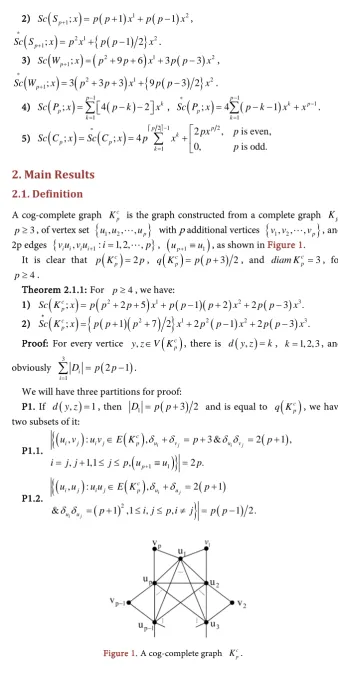
2.1. Definition

A cog-complete graph c p

K is the graph constructed from a complete graph Kp, 3

p≥ , of vertex set

{

u u1, 2,,up

}

with p additional vertices

{

v v1, 2,,vp

}

, and

2p edges

{

v u v ui i, i i+1:i=1, 2,,p

}

,

(

up+1≡u1

)

, as shown in Figure 1.

It is clear that p K

( )

cp =2p,

( )

(

3 2

)

c p

q K = p p+ , and c 3

p

diam K = , for

4

p≥ .

Theorem 2.1.1: For p≥4, we have:

1)

(

) (

2

)

1

(

)(

)

2

(

)

3

; 2 5 1 2 2 3 .

c p

Sc K x = p p + p+ x +p p− p+ x + p p− x

2)

(

)

{

(

)

(

2

)

}

1 2

(

)

2

(

)

3

; 1 7 2 2 1 2 3 .

c p

Sc K x p p p x p p x p p x

∗

= + + + − + −

Proof: For every vertice y z, ∈V K

( )

c_p , there is d y z

( )

, =k, k=1, 2, 3, and

obviously 3

(

)

1

2 1

i i

D p p

=

= −

∑

.

We will have three partitions for proof:

P1. If d y z

( )

, =1, then D₁ = p p

(

+3 2

)

and is equal to

( )

c p

q K , we have

two subsets of it:

P1.1.

{

(

)

( )

(

)

(

1 1

)

}

, : , 3 & 2 1 ,

, 1,1 , 2 .

i j i j

c

i j i j p u v u v

p

u v u v E K p p

i j j j p u u p

δ δ δ δ

+

∈ + = + = +

= + ≤ ≤ ≡ =

P1.2.

{

(

)

( )

(

)

(

)

2

}

(

)

, : , 2 1

& 1 ,1 , , 1 2.

i j

i j

c

i j i j p u u

u u

u u u u E K p

p i j p i j p p

δ δ

δ δ

[image:3.595.195.534.61.736.2]

∈ + = + = + ≤ ≤ ≠ = −

Figure 1. A cog-complete graph c

p

DOI: 10.4236/oalib.1105625 4 Open Access Library Journal P2. If d y z

( )

, =2, then D2 = p p

(

−1

)

, we have two subsets of it:

P2.1.

{

(

v vi, i+1

)

:δvi +δvi+1 =4 &δ δvi vi+1 =4,1≤ ≤i p v,

(

p+1≡v1

)

}

= p.

P2.2.

{

(

)

( )

(

)

(

1 1

)

}

(

)

, : , 3 & 2 1 ,

1 , , , 1 2 .

i j i j

c

i j i j p v u v u

p

v u v u E K p p

i j p i j j u u p p

δ δ δ δ

+

∉ + = + = +

≤ ≤ ≠ + ≡ = −

P3. If d y z

( )

, =3, then D3 = p p

(

−3 2

)

, we have:

(

)

{

}

{

(

)

}

(

)

1

, : 4 & 4,1 , , 0,1 ,

3 2.

i j i j

i j v v v v p

v v i j p i j v v

p p

δ +δ = δ δ = ≤ ≤ − ≠ −

= −

From P1 - P3, we have:

(

c_;

) (

2 _{2 5}

)

1

(

₁

)(

₂

)

2 ₂

(

₃

)

3_.

p

Sc K x = p p + p+ x +p p− p+ x + p p− x

(

)

{

(

)

(

)

}

(

)

(

)

*

2 1 2 2 3

; 1 7 2 2 1 2 3 .

c p

Sc K x = p p+ p + x + p p− x + p p− x

Corollary 2.1.2: For p≥4, we have: 1)

( ) (

c ₃ 2 _{10 17}

)

p

Sc K = p p + p− .

2)

( ) (

3 2

)

9 11 29 2

c p

Sc K p p p p

∗

= + + − .

Corollary 2.1.3: For p≥4, we have: 1) 101

( )

(

6 23 4

)

7

c p

Sc K p

≤ < + .

2) 13

( ) (

2

)

15 4 38 63 16

14

c p

Sc K p p

∗

≤ < + + .

Remark 2.1.4:

1)

(

)

1 2

3; 60 30

c

Sc K x = x + x .

2)

(

)

1 2

3; 96 36

c

Sc K x x x

∗

= + _.

2.2. Definition A cog-star graph 1

c p

S + is the graph constructed from a star graph, Sp+1, p≥3,

of vertex set

{

u u0, 1,,up−1,up

}

with p additional vertices

{

v v1, 2,,vp−1,vp

}

,

[image:4.595.281.464.550.701.2]

and edges

{

v u v ui i, i i+1:i=1, 2,,p

}

,

(

up+1≡u1

)

, as shown in Figure 2.

Figure 2. A cog-star graph 1

DOI: 10.4236/oalib.1105625 5 Open Access Library Journal It is clear that

( )

1 2 1

c p

p S ₊ = p+ ,

( )

c₁ 3

p

q S ₊ = p, diam Spc+₁=4 for p≥4.

Theorem 2.2.1: For p≥4, we have:

1)

(

)

(

)

1

(

)

2

(

)

3

(

)

4

1; 13 4 3 5 2 2 3 .

c p

Sc S ₊ x = p p+ x +p p+ x + p p− x + p p− x

2)

(

)

(

)

1

{

(

)

}

2

(

)

3

(

)

4

1; 3 4 13 1 2 6 2 2 3

c p

Sc S x p p x p p x p p x p p x

∗

+ = + + − + − + −

Proof: For every vertice ,

( )

1

c p

y z∈V S ₊ , there is d y z

( )

, =k, k=1, 2, 3, 4,

and obviously 4

(

)

1

2 1

i i

D p p

=

= +

∑

.

We will have four partitions for proof:

P1. If d y z

( )

, =1, then D1 =3p and is equal to

( )

1

c p

q S ₊ , we have two

subsets of it:

P1.1.

{

(

0,

)

: 0

( )

1 , _{0 i} 3 & _{0 i} 3 ,1

}

.

c

i i p u u u u

u u u u ∈E S + δ +δ = +p δ δ = p ≤ ≤i p = p

P1.2.

{

(

)

( )

(

)

}

1

1 1

, : , 5 & 6,1 ,

, 1, 2 .

i j i j

c

i j i j p v u v u

p

v u v u E S i p

j i i u u p

δ δ δ δ

+

+

∈ + = = ≤ ≤

= + ≡ =

P2. If d y z

( )

, =2, then D₂ = p p

(

+3 2

)

, we have three subsets:

P2.1.

{

(

,

)

: 6 & 9,1 , ,

}

(

1 2.

)

i j i j

i j u u u u

u u δ +δ = δ δ = ≤i j≤ p i≠ j = p p−

P2.2.

{

(

u v0, i

)

:δu0 +δvi = +p 2 &δ δu0 vi =2 ,1p ≤ ≤i p

}

= p.

P2.3.

{

(

v vi, i+1

)

:δvi +δvi+1 =4 &δ δvi vi+1 =4,1≤ ≤i p v,

(

p+1≡v1

)

}

= p. P3. If d y z

( )

, =3, then D3 = p p

(

−2

)

, we have:

(

)

{

}

{

(

)

}

(

)

1

, : 5 & 6,1 , , 0,1 ,

2 .

i j i j

i j u v u v p

u v i j p i j u v

p p

δ +δ = δ δ = ≤ ≤ − ≠ −

= −

P4. If d y z

( )

, =4, then D4 = p p

(

−3 2

)

, we have:

(

)

{

}

{

(

)

}

(

)

1

, : 4 & 4,1 2, 2 ,

3 2.

i j i j

i j v v v v p

v v i p i j p v v

p p

δ +δ = δ δ = ≤ ≤ − + ≤ ≤ −

= −

From P1 - P4, we have:

(

)

(

)

1

(

)

2

(

)

3

(

)

4

1; 13 4 3 5 2 2 3 .

c p

Sc S ₊ x = p p+ x +p p+ x + p p− x + p p− x

(

)

(

)

{

(

)

}

(

)

(

)

*

1 2 3 4

1; 3 4 13 1 2 6 2 2 3 .

c p

Sc S + x = p p+ x + p p− x + p p− x + p p− x

Corollary 2.2.2: For p≥4, we have: 1)

( )

1

(

32 35

)

c p

Sc S ₊ = p p− .

2)

( )

1 7

(

6 7

)

c p

Sc S p p

∗

+ = − .

Corollary 2.2.3: For p≥4, we have:

1)

( )

1

1

10 16

3

c p

Sc S +

≤ < .

2)

( )

1

2

13 21

9

c p

Sc S ∗

+

≤ < .

DOI: 10.4236/oalib.1105625 6 Open Access Library Journal

1)

(

)

1 2 3

4; 48 45 15

c

Sc S x = x + x + x .

2)

(

)

1 2 3

4; 63 57 18

c

Sc S x x x x

∗

= + + .

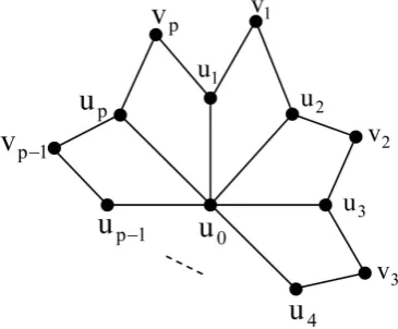
2.3. Definition A cog-wheel graph 1

c p

W + is the graph constructed from a wheel Wp+1, p≥3,

of order p+1, with vertex set

{

u u u₀, ₁, ₂,,u_p

}

and with p additional vertices

1, 2, , p

[image:6.595.207.539.291.706.2]

v v  v , and edges

{

v u v ui i, i i+₁:i=1, 2,,p

}

,

(

up+1≡u1

)

, as shown in

Figure 3.

It is clear that

(

1

)

2 1

c p

p W ₊ = p+ ,

(

c₁

)

4

p

q W ₊ = p, diamWpc+₁=4 for p≥6.

Theorem 2.3.1: For p≥6, we have:

1)

(

)

(

)

1

(

)

2

(

)

3

(

)

4

1; 29 6 5 7 24 2 5 .

c p

Sc W ₊ x = p p+ x +p p+ x +p p− x + p p− x

2)

(

)

(

)

{

(

)

}

(

)

(

)

1 2 3

1

4

; 5 9 29 27 2 / 2 5 18

2 5 .

c p

Sc W x p p x p p x p p x

p p x

∗

+ = + + − + −

+ −

Proof: For every vertice ,

( )

1

c p

y z∈V W ₊ , there is d y z

( )

, =k, k=1, 2, 3, 4,

and obviously 4

(

)

1

2 1

i i

D p p

=

= +

∑

.

We will have four partitions for proof:

P1. If d y z

( )

, =1, then D1 =4p and is equal to

(

1

)

c p

q W ₊ , we have three

subsets of it:

P1.1.

{

(

0,

)

: 0

( )

1 , _{0 i} 5 & _{0 i} 5 ,1

}

.

c

i i p u u u u

u u u u ∈E W + δ +δ = +p δ δ = p ≤ ≤i p =p

P1.2.

{

(

)

(

)

(

)

}

1

1

1 1 1

1 1

, : , 10

& 25,1 , .

i i

i i

c

i i i i p u u

u u p

u u u u E W

i p u u p

δ δ

δ δ

+

+

+ + +

+

∈ + =

= ≤ ≤ ≡ =

P1.3.

{

(

)

( )

(

)

}

1

1 1

, : , 7

& 10,1 , , 1, 2 .

i j

i j

c

i j i j p v u

v u p

v u v u E W

i p j i i u u p

δ δ

δ δ

+

+

∈ + =

= ≤ ≤ = + ≡ =

P2. If d y z

( )

, =2, then D2 = p p

(

+5 2

)

, we have five subsets

P2.1.

{

(

)

}

(

)

{

1

}

(

)

, : 10 & 25,1 2, 2

, 3 2.

i j i j

i j u u u u

p

u u i p i j p

u u p p

δ +δ = δ δ = ≤ ≤ − + ≤ ≤

− = −

Figure 3. A cog-wheel graph 1

c p

DOI: 10.4236/oalib.1105625 7 Open Access Library Journal P2.2.

{

(

u v0, i

)

:δu0 +δvi = +p 2 &δ δu0 vi =2 ,1p ≤ ≤i p

}

= p.

P2.3.

{

(

u vi, i+1

)

:δui +δvi+1 =7 &δ δui vi+1 =10,1≤ ≤i p v,

(

p+1≡v1

)

}

= p.

P2.4.

{

(

)

}

(

) (

)

{

}

2 2

2

1 1 2

, : 7 & 10, 3

, , , .

i i i i

i i u v u v

p p

u v i p

u v u v p

δ δ ₋ δ δ ₋

−

−

+ = = ≤ ≤ =



P2.5.

{

(

v vi, i+1

)

:δvi +δvi+1 =4 &δ δvi vi+1 =4,1≤ ≤i p v,

(

p+1≡v1

)

}

= p. P3. If d y z

( )

, =3, then D3 = p p

(

−3

)

, we have two subsets:

P3.1.

(

)

{

(

)

}

{

(

)

}

(

)

1 1

, : 7 & 10, 3 ,1 , 2, 1,

, 1, , : 1, 2, 2 3

4 .

i j i j

i j u v u v

p i j

u v i p j p j i i

i i v v u v i i j p i

p p

δ δ δ δ

+

+ = = ≤ ≤ ≤ ≤ ≠ − −

+ ≡ = + ≤ ≤ + −

= −



P3.2.

(

)

(

) (

)

{

v vi, i+2 :δvi +δvi+2 =4 &δ δvi vi+2 =4,1≤ ≤i p v, p+1≡v1 , vp+2 ≡v2

}

= p. P4. If d y z

( )

, =4, then D4 = p p

(

−5 2

)

, we have:

(

)

{

(

) (

)

}

{

(

)

}

(

)

1 1 2 2

, : 4 & 4, 3 ,1 , 2, 1, , 1,

2, , , : 1, 2, 3 3

5 2.

i j i j

i j v v v v

p p i j

v v i p j p j i i i i

i v v v v v v i i j p i

p p

δ δ δ δ

+ +

+ = = ≤ ≤ ≤ ≤ ≠ − − +

+ ≡ ≡ = + ≤ ≤ + −

= −



From P1 - P4, we have:

(

)

(

)

1

(

)

2

(

)

3

(

)

4

1; 29 6 5 7 24 2 5 .

c p

Sc W ₊ x = p p+ x +p p+ x +p p− x + p p− x

(

)

(

)

{

(

)

}

(

)

(

)

*

1 2 3

1

4

; 5 9 29 27 2 2 5 18

2 5 .

c p

Sc W x p p x p p x p p x

p p x

+ = + + − + −

+ −

Corollary 2.3.2: For p≥6, we have: 1)

(

1

)

(

42 73

)

c p

Sc W ₊ = p p− .

2)

( )

1 2

(

36 65

)

c p

Sc W p p

∗

+ = − .

Corollary 2.3.3: For p≥6, we have:

1)

( )

1

10

13 21

13

c p

Sc W +

≤ < .

2)

( )

1

3

23 36

13

c p

Sc W ∗

+

≤ < .

Remark 2.3.4:

1)

(

)

1 2 3

6; 170 175 55

c

Sc W x = x + x + x ,

(

)

1 2 3

5; 132 116 8

c

Sc W x = x + x + x ,

(

)

1 2

4; 96 48

c

Sc W x = x + x .

2)

(

)

1 2 3

6; 350 295 70

c

Sc W x x x x

∗

= + + ,

(

)

1 2 3

5; 260 178 8

c

Sc W x x x x

∗

= + + ,

(

)

1 2

4; 180 60

c

Sc W x x x

∗

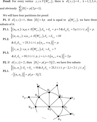
DOI: 10.4236/oalib.1105625 8 Open Access Library Journal 2.4. Definition

A saw graph c p

P is a path of order p, say

{

u u1, 2,,up

}

, with p−1

addition-al vertices

{

v v1, 2,,vp−1

}

and edges

{

v u v ui i, i i+1:i=1, 2,,p−1

}

as depicted

in Figure 4.

It is clear

( )

c 2 1

p

p P = p− ,

( )

c 3

(

1

)

p

q P = p− and c 1

p

diam P = −p , for p≥2. Theorem 2.4.1: For p≥5, we have:

1)

(

)

(

)

1 3

(

)

2 1

2

; 4 5 7 8 3 3 1 40 16 .

p

c k p p

p

k

Sc P x p x p k x x x

−

− −

=

= − +

∑

− − + +

2) *

(

)

(

)

1 3

(

)

2 1

2

; 8 4 7 12 3 3 2 48 16 .

p

c k p p

p

k

Sc P x p x p k x x x

−

− −

=

= − +

∑

− − + +

Proof:

For every vertice y z, ∈V P

( )

_pc , there is d y z

( )

, =k, 1≤ ≤ −k p 1, and

ob-viously 1

(

)(

)

1

2 1 1

p i i

D p p

−

=

= − −

∑

.

We will have four partitions for proof:

P1. if d y z

( )

, =1, then D₁ =3

(

p−1

)

and is equal to

( )

c p

q P , we have five

subsets of it:

P1.1.

{

(

, 1

)

: 1

( )

, i i1 6, i i1 8, 1, 1

}

2.

c

i i i i p u u u u

u u+ u u+ ∈E P δ +δ ₊ = δ δ ₊ = i= p− =

P1.2.

{

(

)

(

)

( )

( ) ( )

( ) ( )

}

1 1 1

1 1 1

1, 1 , , 1 : 1 1, 1 , 4,

4 2.

p p

p p

c

p p p p p u u v v

u u v v

u v u v u v u v E P δ δ

δ δ

−

−

− − ∈ + =

= =

P1.3.

{

(

, 1

)

: 1

( )

, i i1 6, i i1 8, 2 1

}

2.

c

i i i i p u v u v

u v− u v− ∈E P δ +δ ₋ = δ δ ₋ = ≤ ≤ −i p = −p

P1.4.

{

(

u vi, i

)

:u vi i∈E P

( )

pc ,δu_i+δv_i =6,δ δu_i v_i =8, 2≤ ≤ −i p 1

}

= −p 2.

P1.5.

(

)

( )

{

, 1 : 1 , i i1 8, i i1 16, 2 2

}

3.

c

i i i i p u u u u

u u₊ u u₊ ∈E P δ +δ ₊ = δ δ ₊ = ≤ ≤ −i p = −p

P2. if d y z

( )

, =k, 2≤ ≤ −k p 3, then

(

)(

)

3

2

2 4 1

p k k

D p p

−

=

= − +

∑

, we have six

subsets of it:

P2.1.

{

(

)

}

(

)

{

}

1 1 1 1

1 1

1 1

1

, : 6, 8

, : 4, 4 2.

k k

k k

k u u u u

k u v u v

u u

u v

δ δ δ δ

δ δ δ δ

+ +

+ + = =

+ = = =



P2.2.

{

(

)

}

(

)

{

}

, : 6, 8

, : 4, 4 2.

p p k p p k

p p k p p k

p p k u u u u

p p k u v u v

u u

u v

δ δ δ δ

δ δ δ δ

− −

− −

−

−

+ = =

+ = = =

[image:8.595.203.542.105.755.2]



Figure 4. A saw graph c

p

DOI: 10.4236/oalib.1105625 9 Open Access Library Journal

P2.3.

{

(

,

)

: 8, 16, 2 1

}

2.

i k i i k i

i k i u u u u

u u i p k

p k

δ δ ₊ δ δ ₊

+ + = = ≤ ≤ − −

= − −

P2.4.

{

(

u vi, k i+ −1

)

:δui +δvk i+ −1 =6,δ δui vk i+ −1 =8, 2≤ ≤ −i p k

}

= − −p k 1.

P2.5.

{

(

1, 1

)

: 1 1 6, 1 1 8, 2

}

1.

p i p k i p i p k i

p i p k i u v u v

u v i p k

p k

δ _{− +} δ _{− − +} δ _{− +}δ _{− − +}

− + − − + + = = ≤ ≤ −

= − −

P2.6.

{

(

v vi, i k+ −1

)

:δvi +δvi k+ −1 =4,δ δvi vi k+ −1 =4,1≤ ≤ −i p k

}

= −p k. P3. if d y z

( )

, = −p 2 then D_p−2 =8, we have six subsets of it: P3.1.

{

(

u ui, p i+ −2

)

:δui +δup i+ −2 =6,δ δui up i+ −2 =8,i=1, 2

}

=2.

P3.2.

{

(

u v1, p−2

)

:δu1+δvp−2 =4,δ δu1 vp−2 =4

}

=1.

P3.3.

{

(

u vp, 2

)

:δup +δv2 =4,δ δup v2 =4

}

=1.

P3.4.

{

(

u v2, p−1

)

:δu₂ +δv_p−₁ =6,δ δu₂ v_p−₁ =8

}

=1.

P3.5.

{

(

up−1,v1

)

:δup−1+δv1 =6,δ δup−1 v1 =8

}

=1.

P3.6.

{

(

v vi, p i+ −3

)

:δvi +δvp i+ −3 =4,δ δvi vp i+ −3 =4,i=1, 2

}

=2. P4. if d y z

( )

, = −p 1 then Dp−1 =4, we have four subsets of it:

P4.1.

{

(

u u1, p

)

:δu1+δup =4,δ δu1 up =4

}

=1.

P4.2.

{

(

u v1, p−1

)

:δu1+δvp−1=4,δ δu1 vp−1=4

}

=1.

P4.3.

{

(

u vp, 1

)

:δup+δv1 =4,δ δup v1 =4

}

=1.

P4.4.

{

(

v v1, p−1

)

:δv1+δvp−1 =4,δ δv1 vp−1 =4

}

=1. From P1 - P4, we have:

(

)

(

)

3

(

)

2 1

2

; 4 5 7 8 3 3 1 40 16 .

p

c k p p

p

k

Sc P x p x p k x x x

−

− −

=

= − +

∑

− − + +

(

)

(

)

3

(

)

*

2 1

2

; 8 4 7 12 3 3 2 48 16 .

p

c k p p

p

k

Sc P x p x p k x x x

−

− −

=

= − +

∑

− − + +

Corollary2.4.2: For p≥5, then:

1)

( )

(

)(

)

2

4 1 1

c p

Sc P = p+ p− .

2) *

( )

(

)

2

6 1

c p

Sc P = p p− .

Corollary2.4.3: For p≥5, then:

1) 102

( )

2 1

3

c p

Sc P p

≤ ≤ + _.

2) 131 *

( )

3 2

(

1 2

)

3

c p

Sc P p

≤ < − .

Remark 2.4.4:

1)

(

)

1 2

3; 32 16

c

Sc P x = x + x ,

(

)

1 2 3

4; 52 40 16

c

Sc P x = x + x + x .

2) *

(

)

1 2

3; 40 16

c

Sc P x = x + x ,

(

)

*

1 2 3

4; 72 48 16

c

DOI: 10.4236/oalib.1105625 10 Open Access Library Journal 2.5. Definition

A Cog-Cycle is a graph Ccp,p≥3 obtained from a cycle graph

{

1, 2, , , 1

}

p p

C = u u  u u with p additional vertices

{

v v₁, ₂,,v_p

}

, and edges

(

)

{

v u v ui i, i i+1:i=1, 2,, ,p u1≡up+1

}

as shown in Figure 5. It’s clear that

( )

c 2 ,

( )

c 3

p p

p C = p q C = p, and

(

)

(

)

2 1, is even 4,

1 2 , is odd 3.

c p

p p p

diam C

p p p

+ ≥

 = 

+ ≥



Theorem 2.5.1: For p≥6, then:

1)

(

)

2 21 2 1

2 2

1 1

2

10 , is even,

; 20 24 2

12 5 , is odd.

p p p

p p

C k

p

k

x x p

Sc C x px p x p

x x p

− +

 − +

   

=

 ₊



= + +

 ₊



∑

2)

(

)

2 21 2 1

2 2

1 1

*

2

14 , is even,

; 32 36 2

18 6 , is odd.

p p p

p p

c k

p

k

x x p

Sc C x px p x p

x x p

− +

 − +

   

=

 ₊



= + +

 ₊



∑

Proof: For every vertice y z, ∈V C

( )

c_p , there is d y z

( )

, =k, 1 1 2

p k  

≤ ≤_{ }+

  ,

and obviously 2

(

)

1

1

2 1

p

i i

D p p

 +    

=

= −

∑

. We will four partitions for proof: P1. if d y z

( )

, =1, then Di =3p and is equal to

( )

c p

q C . We have three

subsets of it: P1.1.

(

, 1

)

: 1

( )

, _{i i1} 8, _{i i1} 16,1 ,

(

1 1

)

.

c

i i i i p u u u u p

u u+ u u+ ∈E C δ +δ ₊ = δ δ ₊ = ≤ ≤i p u + ≡u = p

P1.2.

{

(

,

)

:

( )

, 6, 8,1

}

.

i i i i

c

i i i i p u v u v

u v u v ∈E C δ +δ = δ δ = ≤ ≤i p = p P1.3.

(

)

( )

(

)

{

1, : 1 , i1 i 6, i1 i 8,1 , 1 1

}

c

i i i i p u v u v p

u+ v u v+ ∈E C δ ₊ +δ = δ δ₊ = ≤ ≤i p u + ≡u =p

P2. If d y z

( )

, =k, 2 1 2

p k  

≤ ≤_{ }−

  , then

2 1

2

4

p

k k

D p

 −    

=

=

∑

. We have four

[image:10.595.195.539.81.719.2]

sub-sets of it:

Figure 5. A Cog-Cycle Graph c

p

DOI: 10.4236/oalib.1105625 11 Open Access Library Journal when ui moving to vj clockwise.

P2.1.

{

(

u ui, j

)

:δu_i +δu_j =8,δ δu_i u_j =16,1≤i j, ≤p i, − =j k p, −k

}

= p.

P2.2.

{

(

u vi, j

)

:δu_i +δv_j =6,δ δu_i v_j =8,1≤i j, ≤ p i, − = −j k 1,p− +k 1

}

= p.

when ui moving to vj reversed clockwise.

P2.3.

{

(

u vi, j

)

:δu_i+δv_j =6,δ δu_i v_j =8,1≤i j, ≤ p i, − =j k p, −k

}

= p.

P2.4.

{

(

v vi, j

)

:δv_i +δv_j =4,δ δv_i v_j =4,1≤i j, ≤ p i, − = −j k 1,p− +k 1

}

= p.

P3. If d y z

( )

, = _p 2_, when p is even, then D_p2 =7p 2, we have four subsets of it:

P3.1.

{

(

u ui, i p+ 2

)

:δui +δup/2 =8,δ δui up2 =16,1≤ ≤i p 2

}

= p 2. when ui moving to vj clockwise.

P3.2.

(

)

(

)

(

)

{

}

(

)

(

)

(

)

{

}

, : 6, 8,1 1 2 1, 2 1

, : 6, 8, 2 2 , 2 1

.

i j i j

i j i j

i j u v u v

i j u v u v

u v i p j p i

u v p i p j i p

p

δ δ δ δ

δ δ δ δ

+ = = ≤ ≤ + + = + − + = = + ≤ ≤ = − − =



when ui moving to vj reversed clockwise.

P3.3.

(

)

(

)

{

}

(

)

(

)

(

)

{

}

, : 6, 8,1 2 , 2

, : 6, 8,1 2 , 2

.

i j i j

i j i j

i j u v u v

i j u v u v

u v i p j p i

u v p i p j i p

p

δ δ δ δ

δ δ δ δ

+ = = ≤ ≤ = + + = = + ≤ ≤ = − =



P3.4.

(

)

(

)

(

)

{

}

(

)

(

)

(

)

{

}

, : 4, 4,1 2 1, 2 1

, : 4, 4, 2 2 , 2 1

.

i j i j

i j i j

i j v v v v

i j v v v v

v v i p j i p

v v p i p j i p

p

δ δ δ δ

δ δ δ δ

+ = = ≤ ≤ + = + − + = = + ≤ ≤ = − − =



when p is odd, then D(p−1 2) =4p, we have four subsets of it:

P’3.1.

(

,

)

: 8, 16,1 , , , .

2 2

i j i j

i j u u u u

p p

u u δ δ δ δ i j p i j p

 _{+ = = ≤ ≤ − =}    ₌

 _{   }

   

 

when ui moving to vj clockwise.

P’3.2.

(

)

(

)

(

)

{

}

(

)

(

)

(

)

{

}

, : 6, 8,1 3 2 , 3 2

, : 6, 8, 5 2 , 3 2

.

i j i j

i j i j

i j u v u v

i j u v u v

u v i p j i p

u v p i p j i p

p

δ δ δ δ

δ δ δ δ

+ = = ≤ ≤ + = + − + = = + ≤ ≤ = − + =



when ui moving to vj reversed clockwise.

P’3.3.

(

)

(

)

(

)

{

}

(

)

(

)

(

)

{

}

, : 6, 8,1 1 2 , 1 2

, : 6, 8, 1 2 , 1 2

.

i j i j

i j i j

i j u v u v

i j u v u v

u v i p j i p

u v p i p j i p

p

δ δ δ δ

δ δ δ δ

+ = = ≤ ≤ − = + + + = = + ≤ ≤ = − − =



P’3.4.

(

)

(

)

(

)

{

}

(

)

(

)

(

)

{

}

, : 4, 4,1 3 2 , 3 2

, : 4, 4, 5 2 , 3 2

.

i j i j

i j i j

i j v v v v

i j v v v v

v v i p j i p

v v p i p j i p

p

δ δ δ δ

δ δ δ δ

+ = = ≤ ≤ + = + − + = = + ≤ ≤ = − − =

DOI: 10.4236/oalib.1105625 12 Open Access Library Journal P4. If d y z

( )

, =_p 2_+1, when p is even then D_1+p2 = p 2, we have:

(

)

{

v vi, i p+ 2 :δvi +δvi p+ 2 =4,δ δvi vi p+ 2 =4,1≤ ≤i p 2

}

= p 2.

when p is odd then D(p+1 2) =2p, we have two subsets of it:

P4.1.

(

)

(

)

(

)

{

}

(

)

(

)

(

)

{

}

, : 6, 8,1 1 2 , 1 2

, : 6, 8, 3 2 , 1 2

.

i j i j

i j i j

i j u v u v

i j u v u v

u v i p j i p

u v p i p j i p

p

δ δ δ δ

δ δ δ δ

+ = = ≤ ≤ + = + − + = = + ≤ ≤ = − + =



P4.2.

(

)

(

)

(

)

{

}

(

)

(

)

(

)

{

}

, : 4, 4,1 1 2 , 1 2

, : 4, 4, 3 2 , 1 2

.

i j i j

i j i j

i j v v v v

i j v v v v

v v i p j i p

v v p i p j i p

p

δ δ δ δ

δ δ δ δ

+ = = ≤ ≤ + = + − + = = + ≤ ≤ = − + =



From P1 - P4, we have:

(

)

2 2

1 1

2 2

1 2 1

2

10 ; is even,

; 20 24 2

12 5 ; is odd.

p p

p p

p

c k

p

k

x x p

Sc C x px p x p

x x p

− +

+ −

   

=

 ₊



= + +

 ₊



∑

(

)

2 2

1 1

2 2

1 2 1

*

2

14 ; is even,

; 32 36 2

18 6 ; is odd.

p p

p p

p

c k

p

k

x x p

Sc C x px p x p

x x p

− +

+ −

   

=

 ₊



= + +

 ₊



∑

Corollary2.5.2: For p≥6, then: 1)

( ) (

c ₃ 2 _{5 2}

)

p

Sc C = p p + p− .

2)

( )

2 *

2

9 12 4; is even,

2 9 12 5; is odd.

c p

p p p

p Sc C

p p p

 + −

= 

+ −



Corollary2.5.3: For p≥6, then: 1) 124

( )

(

3 7 2

)

11

c p

Sc C p

≤ < + _.

2) 17.7 *

( )

c

(

18 53 8

)

p

Sc C p

< < + . Remark 2.5.4:

1)

(

)

1 2 3

4; 80 80 8

c

Sc C x = x + x + x , Sc C

(

₅c;x

)

=100x1+120x2+50x3.

2) *

(

)

1 2 3

4; 128 112 8

c

Sc C x = x + x + x ,

(

)

*

1 2 3

5; 160 180 60

c

Sc C x = x + x + x .

Conflicts of Interest

The authors declare no conflicts of interest regarding the publication of this paper.

References

[1] Buckley, F. and Harary, F. (1990) Distance in Graphs. Addison-Wesley, New York. [2] Chartrand, G. and Lesniak, L. (1986) Graphs and Digraphs. 2nd Edition,

Wads-worth and Brooks/Cole, Pacific Grove.

DOI: 10.4236/oalib.1105625 13 Open Access Library Journal [4] Diestel, R. (2000) Graph Theory, Electronic. Springer-Verlag, New York.

[5] Diudea, M.V. (2001) QSPR/QSAR Studies by Molecular Descriptors. Nova, Hun-tington, New York.

[6] Diudea, M.V., Gutman, I. and Jantschi, L. (2001) Molecular Topology. Nova, Hun-tington, New York.

[7] Schultz, H.P. (1989) Topological Organic Chemistry 1. Graph Theory and Topolog-ical Indices of Alkanes. The Journal for Chemical Information and Computer scien-tists, 29, 227-228.https://doi.org/10.1021/ci00063a012

[8] Klavžar, S. and Gutman, I. (1997) Wiener Number of Vertex-Weighted Graphs and a Chemical Application. Discrete Applied Mathematics, 80, 73-81.

https://doi.org/10.1016/S0166-218X(97)00070-X

[9] Ahmed, M. and Haitham, N. (2017) Schultz and Modified Schultz Polynomials of Two Operations Gutman’s. International Journal of Enhanced Research in Science, Technology & Engineering, 6, 68-74.https://doi.org/10.11648/j.acm.20170606.14

[10] Ahmed, M. and Haitham, N. (2017) Schultz and Modified Schultz Polynomials of Cog-Complete Bipartite Graphs. Applied and Computational Mathematics, 6, 259-264.https://doi.org/10.11648/j.acm.20170606.14